This article provides full proof formula to calculate Present Discounted Value (PDV) of income.
We know that investment (t) is one of the important determinants of income (y). What determines investment? While deciding the level of investment a firm has to take into account the market rate of interest, r, which is the cost of financing the investment funds.
If investment funds are borrowed then interest rate, r is explicit cost and if funds are owned by the firm itself then it is implicit cost.
There are different alternative projects or schemes, where a firm can make investment. While deciding in which Project to invest, a firm uses another term known as present discounted value. A firm will invest first in a project whose present discounted value (PDV) is the highest. What is this present discounted value? The PDV of any investment project is the value of the stream of future net returns or incomes. R discounted by the rate of interest, r against the cost C of the project.
ADVERTISEMENTS:
This can be computed by using the following formula:
A project may yield net income for tour or ten future years. To calculate the present value of the future net returns or incomes the interest rate, r, is used. For instance if Ram makes investment of Rs. 100 in a project having one year life time which is expected to yield net income of Rs. 110 after one year, Ram would have to decide what is the value of that Rs. 110 at present.
Suppose market interest rate, r, is 10 per cent. Ram knows that he could lend money and receive a 10 per cent return on it. He will jump at the conclusion that Rs. 110 after one year was worth Rs. 100 now. Therefore, Ram may or may not invest Rs. 100 now in exchange for Rs. 110 to be received after one year. There is nothing to gain net. This is how the PDV is calculated for different periods and of different projects.
If it is greater than 100, then there are positive net return and certainly the firm will make investment.
Assumption:
Computation of PDV of any projects rests on the following assumptions:
1. Expected future returns (R’s) do not change. This assumption is based on constant current business conditions.
2. In real world there are several rates of interest prevalent on different bonds and securities. We assume here single generalized rate of interest.
ADVERTISEMENTS:
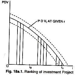
There are various alternative projects or alternative opportunities where the firm can decide to make investment. These various projects can to ranked in order of their PDV’s as shown in the diagram given as under:
With a given value of r the firm will invest in different projects up to a level of ii if there is elastic or unrestricted supply of investment funds. A firm stands to gain by making investment in projects having positive net returns, i.e., with PDV > 0. If investment funds are limited, say up to i0, then investment would be up to i0.
If r rises then the curve will shift leftward due to rise in denominator in the equation. If it falls naturally the PDV curve will shift upward.
In the process the simplest investment model turns out to be:
i = i(r), with i’ < 0.
This shows inverse relationship between r and i. Now the product-market equilibrium condition can be written as:
Y = C[Y – t(Y)] + i (r) + g.

