Equilibrium Income: Determination and Changes (With Diagram)

Equilibrium Income: Determination and Changes!

Determining Equilibrium Income:

The first condition for an equilibrium level of income (output) from equation (2) is Y = C + I + G

Equilibrium income (Y) is the endogenous variable to be determined.

The autonomous components of expenditure, I and G, as also T are exogenous variables determined by factors outside the model.

Consumption is partly autonomous and largely induced expenditure, determined endogenously by the consumption function:

C = a + bY_d = a + bY – bT …(12)

Substituting equation (9) from consumption into the equilibrium condition (2), we can solve for Y̅.:

Y = C + I + G

Y = a + bY – bT + I + G [from equation (12)]

Y – bY = a – bT + I + G

Y(l – b) = a – bT + I + G

Y̅ = 1/1-b x (a-bT + I + G) … (13)

Thus the expression for equilibrium has two parts:

Y̅ = (autonomous expenditure multiplier) x (autonomous expenditure) … (14)

The first term, 1/(1 – b) is called the autonomous expenditure multiplier. Since (1 – b) is the MPS, 1/(1 – b) is the reciprocal of the MPS. Since b is a fraction, the value of the multiplier is some number greater than 1. If, for example, b = 0.5 then 1/(1 – b) = 2. If k= 0.8, 1/(1 – b) = 5.

The expression 1/(1 – b) is called the autonomous expenditure multiplier because every rupee of autonomous expenditure is multiplied by this factor to find out its contribution to equilibrium income.

The second term in the expression is the level of autonomous expenditures. Apart from I and G, there are two other items of autonomous spending, viz., a and -bT. While the first term (a) measures the autonomous component of consumption expenditures, the second term (-bT) measures the autonomous effect of tax collections on aggregate demand, which also works through consumption.

Consumption is partly autonomous and largely induced. Like G and T, the two terms (a and -bT) affect the amount of consumption for a given level of income (Y) and thus the amount aggregate of demand for a given level of income, they are not themselves directly determined by income. They are thus appropriately treated as autonomous factors affecting aggregate demand.

Changes in Equilibrium Income:

Keynes pointed out that any change in autonomous spending would lead to a change in equilibrium income. In the SKM, there are two items of autonomous spending, viz., investment and government expenditure. We may now examine the effect of a change in investment (I) on equilibrium income in SKM, keeping C (which is partly autonomous) and G constant.

By solving for the changes in equilibrium income from equation (21) we get,

A one-unit change in investment changes income by 1/(1 – b) units. If b = 0.8, for example, Y changes by five units for each unit change in investment. Here 1/1 – b is called the multiplier. According to equation (22) the multiplier is the number by which change in autonomous investment has to be multiplied to get the resulting change in income.

According to equation (23), it is the ratio of the two changes, viz., absolute change in Y and absolute change in I. What is the logic of the multiplier? Or, why does income increase by a multiple of the original increase in investment? Let us answer the question in the context of the SKM.

National income is the equilibrium when S + T = I + G. If there is no change in G –and T, national income will rise or fall if S or I changes. Here the initial disturbance is caused by the change in investment. Let us assume that ΔI = 100 units. As some firms make this additional investment expenditure, other firms find that the demand for their goods is rising. So they respond by increasing their output.

In order to produce more output, they require more factors of production. So as they hire (employ) more factors, their factor payments (in the form of wages, rent, interest, and dividends) increase. This implies an increase in the income of the households. Since taxes are assumed to remain fixed an increase in household income implies an equivalent increase in disposable income.

This will lead to an increase in consumption but by less than the amount of increase in income because MPC < 1. This is how the multiplier process is initiated by the initial disturbance created by investment change. The change in consumption is the beginning of the indirect effects of the shock. If ΔI = 100 and b = 0.80, then ΔY = 500 and ΔC = 80.

Since in an interdependent economy one man’s expenditure is another man’s income, the process of income generation continues through a chain of secondary consumption spending. In this case, the new consumption expenditure of 80 units leads to an increase in production and thus generates a second round increase in income for some households of 80 units.

These households will spend 80% of it on consumer goods. So the demand for consumer goods will rise by 64%. Thus the reason that a small increase in autonomous investment leads to a multiple increase in national income is the induced increase in consumption expenditure as income increases.

How large is the multiplier? The size of the multiplier depends on MPC, or its mirror image concept MPS.

With G remaining fixed, the change in equilibrium income can be expressed as:

ΔY = ΔI + ΔC … (24)

If income rises by ΔY, the original equilibrium is disturbed. Equilibrium can be restored (i.e., equality between income and aggregate demand can be maintained) if the absolute increase in income is equal to the increase in primary investment (A/) plus secondary (income-induced) increase in consumption (AC).

So equation (24) can be written as:

ΔY – ΔC = ΔI

or, ΔS = ΔI … (25)

With T and G remaining fixed, equilibrium income can be restored if the increase in income generates enough saving to ensure that new saving is just equated to new investment which disturbed the equilibrium. In this case we have

S + ΔS + T = I + ΔI + G

in terms of equation (5) which is the second way of expressing the condition for equilibrium income.

Since AS equals (1 – b) ΔY, we have from equation (25),

(1 – b)ΔY = ΔI

Or, ΔY/ΔI = 1/1-b = 1/1- MPC = 1/1- MPS …(26)

If, for example, b = 0.8, then MPS = 0.2 and the value of the multiplier is 5. This means that if investment rises by one rupee, income will rise by five rupees. This means that every one-rupee increase in income will generate 20 paise worth of new saving and income has to rise by one rupee to generate an additional new saving of one rupee — which is just sufficient to offset the increase in investment of one rupee.

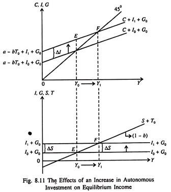
In Fig. 8.11 we illustrate the effect of an increase in autonomous expenditure — autonomous investment to be more specific.

The initial equilibrium income is Y̅₀, when investment is I₁, and government expenditure and taxes are G₀ and T₀, respectively. Now suppose investment increases from I₀ to I₁. As a result the aggregate de­mand schedule shifts up ex­actly by the same amount, from C + I₀ + G₀ to C + I + G₀. The (I + G) schedule in part (b) of Fig. 8.11 also shifts up by the same amount.

National income attains its new equilibrium value Y̅₁, where Y̅₁ = C + I₁, + G₀. From Fig. 8.11, we see that the increase in income is equal to the initial in­crease in investment (shown as an increase in the inter­cept), I₀ to I₁, plus a second­ary (income-induced) in­crease in consumption. This becomes clear from the fact that increase in Y, i.e., ΔY = (Y₁ – Y₀) exceeds the in­crease in investment ΔI = I₁, – I₀.

Thus income increases for two reasons: (1) an ini­tial increase in autonomous investment and (2) a secondary increase in consumption. How much consumption increases as a result of an increase in income (caused by an increase in investment) depends on the MPC. In fact, the slope of the line C + I₀ + G, or line C + I₁ + G, measures MPC, since the slope of the investment schedule and government expenditure schedule is zero. In part (b) we show the increase in saving which occurs when income increases. The increase in saving (ΔS) must be just enough to offset the increase in autonomous investment (ΔI) so that equilibrium is restored at point P after the initial disturbance at point E.

The autonomous expenditure multiplier which is investment multiplier in a two-sector model without government lies at the heart of the simple Keynesian model of income determination. It explains how shifts in investment caused by changes in business expec­tations set off a process of income generation which causes not only investment but also consumption to increase. The investment multiplier shows how shocks to one sector are transmitted throughout the economy.

According to Keynes any increase in autonomous spending will have a multiplier effect.

Examples: