Saving Function of Income: Meaning and Relationship between Saving and Income!
Meaning of Saving Function:
Saving is that part of income which is not spent on current consumption. The relationship between saving and income is called saving function.
Simply put, saving function (or propensity to save) relates the level of saving to the level of income. It is the desire or tendency of the households to save at a given level of income. Thus, saving (S) is a function (f) of income (Y).
Symbolically,
ADVERTISEMENTS:
S = f (Y)
Two noteworthy features of saving function are:
(i) Saving can be negative (-) at zero or low level of income and (ii) As Income increases, savings also increase but more than the increase in income
Remember, saving is residual income of households that is left after consumption.
ADVERTISEMENTS:
Algebraically:
S = Y-C
Saving function equation:
As saving function is corollary of consumption function, we can derive the corresponding saving function from consumption function equation C = C + bY by substituting it in the equation S = Y – C as shown below.
Where C = Autonomous consumption (- C represents dissaving which is needed to finance autonomous consumption. Clearly, at zero level of income, amount of autonomous consumption = Amount of dissaving.), b = MPC (so that 1 – b represents MPS, i.e.. Marginal propensity to save), Y = Income.
For example, the saving equation S = – 30 + (1- 0.75) Y means – 30 is dissaving (or autonomous saving that needs to take place to finance autonomous consumption). As income increases, 0.25 (= 1 – 0.75) or 25% of additional income is saved.
Relationship between Income and Saving:
(i) There is direct relationship between income and saving, i.e., if income increases, saving also increases but by less than increase in income. It means as income increases, proportion of income saved increases (because proportion of income consumed decreases).
(ii) At lower level of income, saving is negative. In the initial stages when there is very low level of income, consumption expenditure is more than income leading to negative saving [i.e., dissaving). For instance, if income is, say, Rs 5,000 and consumption expenditure is, say 6,000, then saving will be negative, i.e., -1000 (= 5000 – 6000). It is called dissaving. Here average propensity to save is negative.
APS = -1000/5000 = -0.2.
Saving Function Curve:
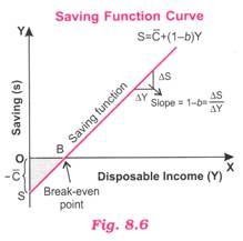
A diagrammatic representation of relationship between income and savings level gives the saving function curve. In Fig. 8.6 saving function curve is a straight line because slope of saving is constant.
The curve slopes upward which depicts direct relationship between income and saving. The savings functions line SS cuts the income line at point B which is called Break-even point because at this point consumption expenditure is equal to income (or savings are zero).
To the left of break-even point, savings are negative (-) indicating consumption being more than income whereas to the right of break-even point, savings are positive (-K) indicating consumption expenditure being less than income. The shaded area reflects dissaving which is equal to the area of autonomous consumption shown as – C in Fig. 8.6.

