Application of Indifference Curve (IC)

In this article we will discuss about the application of Indifference Curve (IC) analysis to solve the problem of analysing the supply of labour of an individual worker.

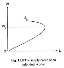
We may apply the indifference curve (IC) analysis to the problem of analysing the supply of labour of an individual worker. We shall see that the labour supply curve of an individual worker may be sloping upward towards right initially and then, as the wage rate (W) rises beyond a certain level, the supply curve may be backward bending. One such curve has been shown in Fig 15.8.

Here, the worker is confronted with two goods, viz., income and leisure. Indifference curves between income and leisure give us the worker’s preference-indifference pattern between the goods. Both these goods are of more-is-better type, i.e., the marginal utilities (MUs) of both the goods are positive. That is why these ICs would be negatively sloped, and higher ICs would represent a higher level of utility.

Also, to get an extra unit of income, the consumer would be willing to forego smaller amounts of leisure to keep his level of utility, unchanged, i.e., the marginal rate of substitution of income for leisure would be diminishing as the consumer goes on substituting income for leisure.

That is why the ICs would be convex to the origin. Also, consistency demands that the ICs would be non-intersecting curves. We shall also assume here that both the goods are normal goods.

Let us now note that the price of Re 1 of income is Re 1. The price of one hour of leisure, on the other hand, is the (hourly) rate of wage (W) itself. This is because, to get one additional hour of leisure, the worker would have to supply one hour less of labour and his income would be less by W.

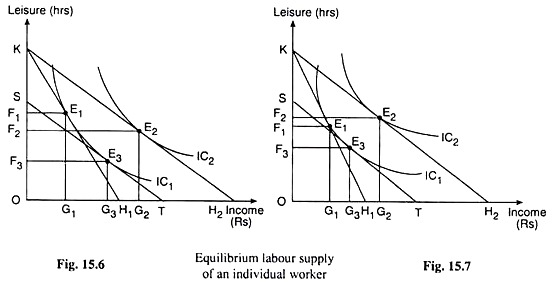
Let us now refer to Fig. 15.6 where the ICs between income and leisure have been given. Let us also note that if the consumer takes zero of income, he may have 24 (OK) hours of leisure and if he takes zero hours of leisure what amount of income he would be able to earn would depend upon W. Let us suppose this amount of income is OH₁.

Therefore, the worker’s budget line here would be the line KH₁. He may have any income-leisure combination on this line including the points K and H₁. The numerical slope of the budget line KH₁ is Ok/OH₁ which is the reciprocal of the price per hour of leisure, OH₁/OK, or, the rate of wage (= W₁, say).

Now, in Fig. 15.6, when W = W, and the budget line is KH₁, the worker is in equilibrium at the point of tangency E₁ on IC₁. At E₁, the worker has OG, of income and OF, of leisure. That is, at W = W₁ the worker supplies KF₁ (= OK – OF₁) hours of labour.

Let us now suppose that W rises from W₁ to W₂, and consequently, the worker’s budget line becomes KH₂. The worker now would be maximising utility at the point of tangency E₂ on a higher IC₁ viz., IC₂ (since his real income has increased), having OG₂ of income and OF₂ of leisure.

That is, at W = W₂, the worker supplies KF₂ (= OK – OF₂) hours of labour. Since KF₂ is greater than KF₁, we have obtained here that as the rate of wage rises, the worker increases his supply of labour. Therefore, here, the worker’s labour supply curve has been obtained to be upward sloping.

In order to understand why the worker’s supply curve has been obtained to be upward sloping (positively sloped), and when his supply curve may be backward bending, we have to break up the total effect (TE) of the rise in W (i.e., of the rise in the price of leisure), which is represented by the movement of his equilibrium point from E₁ to E₂, into a substitution effect (SE) and an income effect (IE).

To obtain the SE, let us allow the worker the rise in W from W₁ to W₂ at the initial equilibrium point E₁, but let us not allow him, for the time being, the conse­quent gain in real income. Under the circumstances, the worker would have a budget line, ST, that would be parallel to KH₂ but tangent to IC, at the point E₃.

The movement from the point E₁ to the point E₃ along IC₁ represents the SE of the change in the relative prices of leisure and income (caused by the rise in W), the worker’s real income remaining constant. At E₃, as compared to the point E₁, the worker would have G₁G₃ more of income and F₁F₃ less of lei­sure—he would substitute the relatively cheaper commodity, income, for the relatively dearer commodity, leisure.

As a result, owing to the SE of the rise in W, the supply of labour would increase from KF₁ to KF₃. However, after isolating the SE from the total effect, let us now allow the worker the gain in his real income which has occurred owing to the rise in W. As a consequence, the worker’s budget line now would shift from ST to KH₂ and his equilibrium point would move from E₃ to E₂, owing to the income effect (IE) of the rise in W.

As a result of this effect, the consumer would have G₃G₂ more of income and F₃F₂ more of leisure. Since his income has increased, he is now having more of both the goods.

However, here the IE-rise in leisure has been less than the SE-fall in leisure, because the worker does not yet think it worth­while to have more of leisure in the net now that his W has increased. So here, there has been a net fall in the amount of leisure and a net increase in the supply of labour by F₁F₂ (= F₁F₃ – F₂F₃) owing to the rise in W.

We have seen above that, owing to a rise in W, if the SE-fall in the amount of leisure is larger than the IE-rise in it, then the supply of labour would rise and the worker’s supply curve would be upward sloping.

Now, if the opposite happens, i.e., if there is a rise in W, and as a result, the IE-rise in leisure is larger than the SE-fall in leisure, then there would be a net rise in leisure and a net fall in the supply of labour. This may happen if W rises beyond a certain level and the worker thinks himself sufficiently rich to have more of leisure in the net.

Since, in this case, as W rises, the supply of labour falls, the worker’s supply curve of labour would be backward bending. This case has been illustrated in Fig. 15.7. In this figure, as we may see, the IE-rise in the amount of leisure (F₂F₃) has been larger than the SE-fall (F₁F₃). So as a result of a rise in W, there has been a net increase in the amount of leisure, i.e., a net fall in the supply of work by F₂F₃ – F₁F₃ = F₁F₂ hours.

The supply curve (S_L) of an individual worker has been shown in Fig. 15.8. As we have analysed above, as W rises initially, the worker’s supply of labour increases. This goes on as long as the magnitude of the IE-rise in the amount leisure is less than the SE- fall.

As W rises beyond W₀, the supply curve becomes backward bending—now, as W rises, supply of labour falls. This happens, because now the magnitude of the IE-rise in the amount of leisure is larger than the SE-fall