Indifference Curves: Definition, Properties and Other Details

Let us make an in-depth study of the definition, diagram, assumptions, properties, budget line, equilibrium and analysis of indifference curve.

Definition:

According to the indifference curve approach, it is not possible for the consumer to say how much utility he derives from the consumption of a commodity, because utility is not a measureable magnitude.

But a consumer can compare two or more combi­nations of goods and say which of them he likes best or whether he likes them all equally well. The Laws of Consumer Demand can be deduced from these preferences.

Suppose a consumer is asked to choose between the following two combinations:

a. 4 apples and 2 oranges

b. 2 apples and 3 oranges

He may prefer a to b or b to a or he may like both combinations equally well. In the last case we say that he is indifferent between them. It is not necessary at this stage to know how much utility is obtained from an apple or an orange. The consumer can compare the relative desirability of, or indifference between, two combinations of goods without knowing the exact amount of “utility” and “satis­faction” obtained from each combination.

The Diagram:

To show how Indifference Curves are constructed let us take the example of a consumer purchasing two goods only, apple and orange. He may prefer apple to orange but if orange becomes relatively cheap he may be induced to eat a few more units of it. If the price of apple becomes much cheaper he may give up orange altogether.

On the other hand, if the price of apple becomes very high he may be forced by lack of means to give up apple. Between these two extremes he will purchase both apple and orange, but will vary the proportions according to relative prices so that he obtains the advantages of small price changes of either commodity. It follows, therefore, that there are more than one combinations of apple and orange which are equally satisfactory to him.

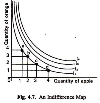
Suppose the following combinations are equivalent:

(a) 1 unit of apple and 4 units of orange

(b) 2 units of apple and 3 units of orange

(c) 3 units of apple and 2 units of orange

(d) 4 units of apple and 1 unit of orange

An Indifference Curve:

These combinations are represented by small circles in Fig. 4.7 where apple is measured on the horizontal axis and orange on the vertical axis. There may be many other such combinations. Let I be a continuous line joining the small circles and other similar points. The curve I₁ is called an indifference curve.

Thus an indifference curve may be defined as a curve which shows combinations of goods which are equivalent to one another. It is a locus of points sharing alternative combinations of apple and orange which give the same satisfaction to the consumer. The consumer has no reason to prefer any of the combinations on the curve to any other on the same curve. He is indifferent as to which of these combinations he uses. Each indifference curve is an equal-utility curve.

Assumptions:

The indifference curve approach is based upon the following assumptions:

1. Non-Satiety:

A rational person will prefer a larger quantity of a good than a smaller amount of it. It is assumed that the consumer has not yet reached the satisfaction point in respect of competition of a good.

2. Transitivity:

The consumer is supposed to be consistent about his tastes and pre­ference. For example if he prefers A to B and B to C then it follows that he also prefers A to C. This assumption is called Transitivity.

3. Diminishing Marginal Substitutability:

Suppose a consumer buys orange and apple. It can be assumed that as more and more of units of apple are substituted for orange, the consumer will be willing to give up fewer and fewer units of orange for additional units of apple. As the quantity of orange consumed increases, more of it will be required to compensate for loss of apple. This follows from the principle that as the consumption of orange increases the desire for it will fall and as the consumption of apple decreases the desire for it will increase.

Therefore, the marginal rate of substitution of orange for apple increases as the quantity of orange increases relatively to apple. Alternatively we can say that the marginal rate of substitution of orange for apple diminishes as the supply of apple diminishes. This is called the Principle of Diminishing Marginal Substitutability. It is assumed that the two goods are not perfect substitutes for one another and that want for the goods are not satiable.

The Principle of Diminishing Marginal Substitutability corresponds to the older law of diminishing marginal utility.

Properties (Characteristics) of Indiffe­rence Curves:

Indifference curves have the following four properties:

1. An indifference curve which lies above and to the right of another shows preferred combinations of the two commodities. This means that indifference curves with larger bundles of goods lie further up and to the right than indifference curves with smaller bundles. In general, movements from left to the right in the commodity space or on the indifference map correspond to increases in utility.

The indifference curves on the Map show different levels of satisfaction or total utility. The higher the position of a curve (i.e., the further out it is on the map) the better it is for consumer. Thus I₃ is superior to I₂,1₂ to I, and so on. The consumer will like to be as high as possible on his indifference map.

2. Indifference Curves Have a Negative Slope:

Let us consider any two combinations of goods on the same indifference curve, such as (h) and (g). Combination (g) has 1 unit of orange (O) more than combination (h). To be equivalent to (h) it must have less apple (A). Hence, when the quantity of one commodity (A) in a combination of two goods increase, the quantity of the other commodity (O) must decline. Therefore, an indifference curve must slope downwards from left to right. This rule follows from assumption 1.

The Marginal Rate of Substitution:

Definition:

The slope of the indifference curve is called the MRS which is the ratio of the marginal utilities of the two commodities. This is expressed as

MRS _x,y = – ΔY /ΔX = MU_x/MU_y

From Fig. 4.7 we find that in (d), (c), (b) and (a), when consumption of A is reduced from 3 to 2 and 1 unit the consumption of O increases from 2 to 4 and 7. The rate at which O is being substituted for A is 1, 2 and 3 units of O per unit of A in the three cases respectively. This rate is called the rate of substitution of O for A. The quantity of O which would just compensate the consumer for the loss of a marginal unit of A is called the marginal rate of substitution of A for O.

3. An Indifference Curve cannot Intersect or Touch Another Indifference Curve:

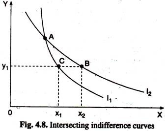
This can be proved by showing that if two indifference curves on the same indifference map intersect, there is logical contradiction (or inconsis­tency). Suppose I₁, and I₂ intersect as in Fig 4.8, then from I₁.

Point A lies on both I₁, and I₂. Since point A I₂ like point C lies on I₁, the consumer is indifferent between A and C. Similarly we can say that the consumer is indifferent between A and B. Applying the transitivity assumption, then we can say that our consumer is indifferent between B and C.

But this is absurd since B contains more X than C while both B and C contain the same amount of Y. We know that more is better (showing higher utility) for the consumer. Hence B should be strictly preferred to C, or B and C cannot show equal level of utility. This explains why indifference curves cannot intersect.

[^..^. Transitivity implies that if A is preferred to B and B is preferred to C then A is preferred to C.]

4. Indifference Curves are Convex to the Origin:

As we proceed downwards along any indi­fference curve the quantity of one commodity consumed (X) increases and that of the other (Y) diminishes. The marginal utility of X therefore, decreases while that of Y increases. It follows that an increasing quantity of X will be required to compensate for the loss of Y. Only a curve convex to the origin can show this fact. This is due to diminishing MRS. The desired rate of commodity Substitute falls as consumer moves along the same indifference curve from left to right.

Conclusion:

Thus it is concluded that

(i) each indifference curve is a distinct line;

(ii) it slopes downwards from left to right and

(iii) it is convex to the origin.

There are, however, certain exceptions to rule 3. Under certain special circumstances an indifference curve may be a straight line or even concave to the origin.

The Budget (Price) Line:

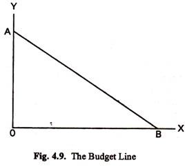
In search for higher utility, the consumer faces a constraint — a limited budget or income. The consumer does not have sufficient funds to purchase all combinations of the two goods. The limits imposed by the budget are shown through the consumer’s budget line. A budget line incorporates information on both the limited income of the consumer to spend and the prices of two purchasable goods.

A budget line is a locus of points showing alternative combinations of two goods that can be purchased with a fixed amount of money income and fixed prices of the two goods.

If we know the budget (or the spending power) of the consumer and his Indifference Map we can find out what quantity of each commodity he will purchase. With the same information we can measure the effect of changes in the prices of commodities and of changes in the income of the consumer.

Suppose a consumer has a fixed income M which he spends on two goods X and Y. Suppose P_x is the price of X and P_y is the price of Y. Let OA be the amount of Y which can be purchased if the whole of the consumer’s income (M) is spent on Y. Then OA x Py = M. Or OA = M/Py. Similarly, let OB be the amount of X which can be purchased with M. Then OB x p_x = M. Join A and B. AB is called the Price Line or the Budget Line or the Consumption-Possibility Line (See Fig. 4.9). The line AB has important characteristics. Every point on it shows a possible distribution of the consumer’s income (M) between X and Y.

The slope of the line is:

A⁰ ÷ OB = M/py ÷ M/px = M/py. py/xy = px/py.

This is known as the price ratio. The equation of the budget line is M = Px. X + Py. Y.

Shift vs. Change in Slope:

A budget line is derived from a given income and given prices. So any change in income or price leads to a new budget line.

If the price of one of the purchasable commodities falls there is a change in the slope of the budget line.

A higher income shifts the budget line outward without changing its slope. A lower income shifts the budget line inward without changing its slope.

Equilibrium of the Consumer:

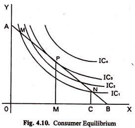
The equilibrium position of the consumer is shown in Fig. 4.10. We assume a consumer with a fixed income M, spending the whole of his income only on two goods, X and Y. AB is the consumption possibility line and IC₁, IC₂ etc. are the indifference curves of the consumer.

The consumer may with M, buy OC of X and NC of Y. In this case he is on indifference curve IC₁. But with the same income M, he can also buy OM of X and PM of Y. In this case he is on IC₃ which denotes a better situation than IC₁. It can be assumed, as a rule of rational behaviour, that the consumer will try to secure the maximum possible satisfaction from his income. He will, therefore, be on the highest indifference curve that he can reach with his income.

A glance at Fig. 4.10 shows that the highest indifference curve the consumer can reach is IC₃ which just touches the con­sumption possibility line AB. AB is the tangent of IC₃ at P. Once the consumer reaches this position he will not shift his purchase pattern, unless his income changes or unless the price of X or of Y becomes different. From this reasoning we can conclude that the equili­brium position of the consumer is at the point where the Consumption Possibility Line is the tangent of an Indifference Curve.

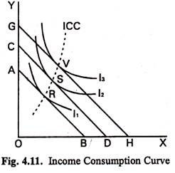
If the consumer is at a point on his consumption-possibility line where it crosses an indifference curve (such as N in Fig. 4.11) he is not getting the maximum possible from his income. He is on a lower indifference curve (IC). He can improve his position by changing his purchases in such a way as to be on P, which is on a higher indifference curve (IC₃). N is, therefore, not a position of equili­brium. If the consumer happens to be at a point like N, he should move towards P, the point of tangency between the consumption- possibility line and an indifference curve.

At the equilibrium point P, the slope of IC₂, is the same as the slope of AB. It can be shown that the slope of IC₃ at any point measures the ratio of substitution between X and Y at that point. Also, the slope of AB = tangent of angle OBA = OA -r OB the ratio between the price of X and the price of Y. Hence, at the position of equilibrium, the ratio between the prices of the two goods just equals the ratio of substitution between them.

Consumer equilibrium refers to a situation in which the consumer obtains the maximum total utility with the consumer’s budget. It occurs where the consumer’s budget line is tangent to the highest attainable indifference curve.

Indifference Curve Analysis and the Demand Curve:

Indifference curve analysis can be used to show why the demand curve usually slopes down. To do this, we will analyse one commo­dity, beer, and assume that consumer income and the price of all other goods remains constant.

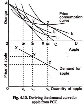
The top part of Figure 4.13 is a conventional indifference curve diagram. The budget line AB shows that the consumer can either buy OB quantity of apples or OA quantity of oranges by spending his total income. When the price of apples falls, the budget line will move to AC and then AD. Originally the consumer would be at position X on indifference curve, but as the price of apple falls the consumer will be able to move to higher indifference curves and I₃. Points X, Y and Z show successive places on the price consumption curve corresponding to changes in the price 6f apples.

The bottom part of the Fig. 4.13 is derived from the top part. In both parts, the horizontal axis shows the quantity of apple which will be bought, but in the bottom part of the diagram, the vertical axis shows the price of apples. This part of the diagram is a conven­tional demand curve diagram. At the original price of apple; the consumer’s preference for apples will be at point X, and quantity q, will be consumed. This is shown in both parts of the Fig. 4.13. The budget line AB also corresponds to a particular price of apples, and is shown in the bottom part as point X.

If the price of apple then falls to that shown by budget line AC, the consumer will maximise satisfaction at point Y, and this corresponds to point Y in the bottom part of the Figure. If we move along the price consumption curve to position Z, we will find the quantity of apple which will be consumed when the budget line becomes AD.

This gives us point Z in the bottom part of the Fig. 4.13. Joining together these points gives us the demand curve for apple, which slopes down to the right. The slope of the curve will depend on the consumer’s preferences as shown in the top part of the diagram. If a fall in the price of apple caused only a few more to be consumed, then OB, OC and OD would be closer together, giving a steeper (inelastic) demand curve.