Separation of Substitution and Income Effects from the Price Effect

In this article we will discuss about Separation of Substitution and Income Effects from the Price Effect.

The Hicksian Method:

Hicks has separated the substitution effect and the income effect from the price effect through compensating variation in income by changing the relative price of a good while keeping the real income of the consumer constant.

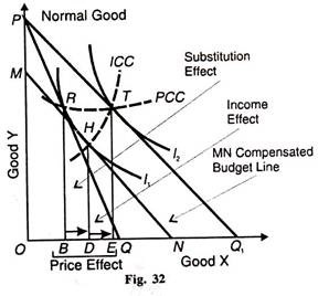
Suppose initially the consumer is in equilibrium at point R on the budget line PQ where the indifference curve I₁, is tangent to it at point R in Figure 32. Let the price of good X fall. As a result, his budget line rotates outward to PQ, where the consumer is in equilibrium at point T on the higher indifference curve I₁ .

The movement from R to T or В to E on the horizontal axis is the price effect of the fall in the price of X. With the fall in the price of X, the consumer’s real income increases.

To make the compensating variation in income in order to isolate the substitution effect, the consumer’s money income is reduced equivalent to PM of Y or Q₁N of X by drawing the budget line MN parallel to PQ₁, so that it is tangent to the original indifference curve I₁ at point H.

The movement from the R to H on the I₁, curve is the substitution effect whereby the consumer increases his purchases of X from В to D on the horizontal axis by substituting X for Y because it is cheaper.

It may be noted that when there is a fall (or rise) in the price of good X, the substitution effect always leads to an increase (or decrease) in its quantity demanded. Thus the relation between price and quantity demanded being inverse, the substitution effect of a price change is always negative, real income being held constant.

This is known as the Slutsky Theorem, named after Slutsky who first stated it in relation to the Law of Demand.

To isolate the income effect from the price effect, return the income which was taken away from the consumer so that he goes back to the budget line PQ₁, and is again in equilibrium at point T on the curve The movement from point H on the lower indifference curve I₁, to point T on the high indifference curve I₂ is the income effect of the fall in the price of good X. By the method of compensating variation in income, the real income of the consumer has increased as a result of the fall in the price of X.

The consumer purchases more of this cheaper good X thus moving on the horizontal axis from D to E. This is the income effect of the fall in the price of a normal good X. The income effect with respect to the price change for a normal good is negative. In the above case, the fall in the price of good X has increased the quantity demanded by DE via the increase in the real income of the consumer.

Thus the negative income effect DE of the fall in the price of good X strengthens the negative substitution effect BD for the normal good so that the total price effect BE is also negative, that is, a fall in the price of good X has led, on both counts, to the increase in its quantity demanded by BE.

This can be written in the form of the Slutsky equation thus:

Price Effect (-) BE = (-) BD (Substitution Effect + (-) DE (Income Effect).

Substitution and Income Effects for an Inferior Good:

If X is an inferior good, the income effect of a fall in the price of X will be positive because as the real income of the consumer increases, less quantity of X will be demanded. This is so because price and quantity demanded move in the same direction.

On the other hand, the negative substitution effect will increase the quantity demanded of X. The negative substitution effect is stronger than the positive income effect in the case of inferior goods so that the total price effect is negative.

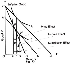
It means that when the price of the inferior good falls, the consumer purchases more of it due to compensating variation in income. The case of X as an inferior good is illustrated Figure 33. Initially, the consumer is in equilibrium at point R where the budget line PQ is tangent to the curve I₁.

With the fall in the price of X, he moves to point T on the budget line PQ, at the higher indifference curve l₂. His movement from R to T or from В to E on the horizontal axis is the price effect. By compensating variation in income, he is in equilibrium at point H on the new budget line MN along the original curve I₁.

The movements from R to H on the I₁, curve is the substitution effect measured horizontally by BD of X. To isolate the income effect, return the increased real income to the consumer which was taken from him so that he is again at point T of the tangency of PQ, line and the curve I₂. The movement from H to T is the income effect of the fall in the price of X and is measured by DE.

This income effect is positive because the fall in the price of the inferior good X leads, via compensating variation in income, to the decrease in its quantity demanded by DE. When the relation between price and quantity demanded is direct via compensating variation in income, the income effect is always positive.

In the case of an inferior good, the negative substitution effect is greater than the positive income effect so that the total price effect is negative. Thus Price Effect (-) BE= (-) BD (Substitution Effect) + DE (Income Effect).

Substitution and Income Effects for a Giffen Good:

A strongly inferior good is a Giffen good, after Sir Robert Giffen who found that potatoes were an indispensable food item for the poor peasants of Ireland. He observed that in the famine of 1848, a rise in the price of potatoes led to an increase in their quantity demanded. Thereafter, a fall in the price led to a reduction in their quantity demanded. This direct relation between prices a quantity demanded in relation to essential food items is called the Giffen paradox.

The reason for such a paradoxical tendency is that when the price of some food articles like bread of mass consumption rises, this is tantamount to a fall in the real income of the consumers who reduce their expenses on more expensive food items, as a result the demand for the bread increases.

Similarly, a fall in the price of bread raises the real income of consumers who substitute expensive food item for bread thereby reducing the demand of bread.

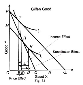
In the case of a Giffen good, the positive income effect is stronger than the negative substitution effect so that the consumer buys less of it when its price falls. This is illustrated in Figure 34. Suppose X is a Giffen good and the initial equilibrium point is R where the budget line PQ is tangent to the indifference curve I₁.

Now the price of X falls and the consumer moves to point T of the tangency between the budget line PQ₁ and the curve I₂ His movement from point R to T is the price effect whereby he reduces his consumption of X by BE.

To isolate the substitution effect, the increased real income due the fall in the price of X is withdrawn from the consumer by drawling the budget line MN parallel PQ. And tangent to the original curve I₁ at point H. As a result, he moves from point R to H along the curve. This is the negative substitution effect which leads him to buy BD more of X with the fall in its price, real income being constant. To isolate the income effect, when the income, which was taken away from the consumer, is returned to him, he moves from point H to T so that he reduces the consumption of X by a very large quantity DE.

This is the positive income effect because with the fall in the price of the Giffen good X, its quantity demanded is reduced by DE via compensating variation in income. In other words, it is positive with respect to price change, that is, the fall in the price of good X leads, via the income effect, to a decrease in the quantity demanded.

Thus in the case of a Giffen good, the positive income effect is stronger than the negative substitution effect so that the total price effect is positive. That is why, the demand curve for a Giffen good has positive slope from left to right upwards. Thus the price effect BE= DE (income effect) + (-) BD (substitution effect).

According to Hicks, a giffen good must satisfy the following conditions:

(i) The consumer must spend a large part of his income on it;

(ii) It must be an inferior good with strong income effect; and

(iii) The substitution effect must be weak. But Giffen goods are very rare which may satisfy these conditions.

Conclusion:

The Hicksian method of decomposing the price effect into the substitution and income effects is defective in that it lacks practical applicability because it is not possible to know exactly how much real income of the consumer should be changed in order to keep him on the original indifference curve. The Slutsky method tries to solve it by taking the apparent real income of the consumer.

The Slutsky Method:

Slutsky explained the income and substitution effects of the price effect by taking the apparent real income of the consumer constant. With the fall in the price of X when the real income of the consumer increases, it is adjusted in such a way that the consumer is in a position to have the same amount of X as before if he likes so that his apparent real income remains constant.

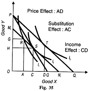
This is because he moves on to a higher indifference curve when the substitution effect takes place. It implies that the Slutsky effect corresponds with rotating budget lines about a point where they intersect each other, such as point R in Fig. 35.

Hicks call this the cost difference method in his A Revision of Demand Theory. Suppose the price of X falls but there is no change in the apparent real income of the consumer. So his increased income due to a price fall is taken from him in such a manner that he may be able to have the original combination of X and Y. The Slutsky effects are depicted in Fig. 35.

The consumer is in equilibrium at point R where the budget line PQ is tangent to I₁, curve. When the price of X falls, PQ₁ becomes the new budget line of the consumer where he is in equilibrium at point T on the indifference curve I₃.

The movement of the consumer from point R to T or from A to D on the horizontal axis is the price effect. With the fall in the price of X, the increased income of the consumer is to be taken away through cost difference so that he may be able to buy the original combination R because it is assumed that his apparent real income remains constant.

For this, the line M₁ N₁ is drawn in such a manner that it passes through point R. This is equivalent to reducing the consumer’s income by PM_X quantity of Y or Q₁ N₁ of X. But on this new budget line M₁ N₁ the consumer is in equilibrium at point S where this line touches the curve I₂.

In reality, with X becoming cheaper relatively to Y, the consumer substitutes X for Y. Thus he sacrifices GH quantity of Y in order to have AC quantity of X. The movement of the consumer from point R to S or from A to С on the horizontal axis is the Slutsky Substitution Effect.

If the withdrawn income of the consumer is returned to him, he will move to point T on the curve I₃. The movement from S to T or from CD on the horizontal axis is the income effect. Thus when the price of X falls, the movement from point R to T or AD is the price effect and the consumer buys AD more of X. The first effect of the price effect is the substitution effect AC which moves the consumer from R to S. Its second effect is the income effect CD which moves him from point S to T.

Slutsky vs. Hicks—Separation of Income and Substitution Effects from Price Effect:

Hicks and Slutsky separate the income and substitution effects of the price effect in different ways. According to Hicks when the price of X falls, the real income of the consumer increases and he remains at the same indifference curve through the substitution effect on the basis of the compensating variation.

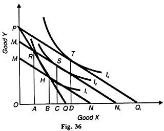
This is due to changes in the relative prices of X and Y so that the increased real income of the consumer is spent in such a manner that he is neither better off nor worse off than before. The consumer moves along the same indifference curve I₁ from one point of equilibrium to the other through the substitution effect, as shown in Figure 36.

On the other hand, the Slutsky substitution effect tells that with the fall in the price of good X, the consumer spends his increased income in such a manner as to buy the original quantities of A and Y if he so desires and there is no change in his apparent real income. But the substitution effect takes place when he moves to the higher indifference curve l₂, as shown in Figure 36.

Figure 36 explains the separation of income and substitution effects of the price effect both in terms of the Hicksian method and the Slutsky method in the case of normal goods. Here PQ is the original budget line where R is the point of equilibrium on indifference curve I₁, at which OA of X and RA of Y are bought by the consumer.

Now with the fall in the price of X, the budget line extends to PQ₁ and the consumer moves to point T on the higher indifference curve l₃.

The movement from R to T is the price effect which shows that the consumer buys AD more of X, as a result of the fall in its price. The price effect is compounded of the substitution effect and the income effect which can be separated in two ways. Following Hicks, we draw a line MN parallel to PQ₁ so that the consumer is at the same real income level on the original indifference curve I₁ at point H on the budget line MN.

The movement from point R to H on the I₁ curve measures the substitution effect. As a result, the consumer buys AB more of X. The remaining increase of BD of X is the result of the income effect from H to T. In terms of the Slutsky method, a new budget line M₁ N₁ is drawn parallel to PQ₁ in such a way that the apparent real income of the consumer remains the same even after the fall in the price of X. If M₁ N₁ passes through point R, the consumer has the same money income to buy combination R as he was buying at the old budget line PQ.

But in reality the consumer prefers the combination S to combination R on the budget line M₁N₁, because point S lies on the budget line which is tangent to a higher indifference curve I₂ than point R which lies on a lower indifference curve I₁. The movement from R to S is the Slutsky substitution effect.

As a result, the consumer buys AC more of X and the movement from S to T or CD of X is the income effect.

Figure 36 also reveals the differences between the two methods of measuring the substitution and income effects. The Hicksian substitution effect is smaller than the Slutsky substitution effect by BC quantity of X. On the other hand, the Hicksian income effect BD is greater than the Slutsky income effect CD.

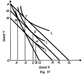
X as an Inferior Good. If X is an inferior good, the income and substitution effects of the price effect when the price of X falls can be explained with the help of Hicks and Slutsky methods. In Figure 37, the movement of the consumer from R to T or A to D on the horizontal axis is the price effect from the points of view of Hicks and Slutsky.

This movement from R to H on the same indifference curve I₁, is due to the Hicksian substitution effect while the movement from R to S is in accordance with the Slutsky substitution effect on the higher curve I₂.

When X is an inferior good and its price falls, the substitution effect is greater than the income effect so that the consumer buys more of X when its price falls. This fact has been classified by both the methods. But the Hicksian substitution effect RH or AB is greater than the Slutsky substitution effect RS or AC. Similarly, the Hicksian income effect BD is greater than the Slutsky income effect CD.

Conclusion:

The Slutsky theorem is a good approximation to keep real income constant and is superior to Hicks’ method. The Slutsky substitution effect provides the consumer greater satisfaction by bringing him on a higher indifference curve, while the Hicksian substitution effect brings him back to the initial level of satisfaction on the original indifference curve.

Hicks himself writes:

“The substitution effect measures the effect of change in relative price, with real income constant, and the income effect measures the effect of the change in real income.”

Hicks’ substitution effect is weak because it is based on the compensating variation in income. In the Slutsky method, income can be calculated equal to cost-difference directly by studying market phenomena and behaviour, whereas the compensating variation in income is difficult to estimate.

In the Slutsky method, the income effect and substitution effect can be computed by observing market prices and quantities bought at those prices without any knowledge of indifference curves even. Hicks again admits that the Slutsky “income effect is peculiarly easy to handle”, while the compensating variation method makes the analysis complex by joining the income effect with the substitution effect.

Thus from a practical viewpoint the Slutsky method is superior to the Hicksian method.