Top 9 Properties of Indifference Curve (With Diagram)

The following points highlight the top nine properties of Indifference Curve.

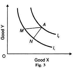
1. A higher indifference curves to the right of another represents a higher level of satisfaction and preferable combination of the two goods. In Figure 3, consider the indifference curves f and I₂ and combinations N and A respectively on them.

Since A is on a higher indifference curve and to the right of N, the consumer will be having more of both the goods X and Y. Even if the two points on these curves are on the same plane as M and A, the consumer will prefer the latter combination, because he will be having more of goods X though the quantity of goods Y is the same.

2. In between two indifference curves there can be a number of other indifference carves, one for every point in the space on the diagram.

3. The numbers I₁, I₂, I₃, I₄, etc. given to indifference curves are absolutely arbitrary. Any numbers can be given to indifference curves. The numbers can be in the ascending order of 1, 2, 4, 6 or 1, 2, 3, 4, etc. Numbers have no importance in the indifference curve analysis.

4. The slope of an indifference curve is negative, downward sloping, and from left to right. It means that the consumer to be indifferent to all the combinations on an indifference curve must leave less units of good Y in order to have more of good X.

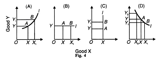
To prove this property, let us take indifference curves contrary to this assumption. In Figure 4 (A) combination В of OX₁+ OY₁ is preferable to combination A which has a smaller amount of the two goods.

Therefore, an indifference curve cannot slope upward from left to right. It is not an iso-utility curve. Similarly, in Figure 4 (B) combination В is preferable to combination A, for combination В has more of X and the same quantity of Y.

So an indifference curve cannot be horizontal. In Figure 4 (C) the indifference curve is shown as vertical and combination В is preferred to A as the consumer has more of Y and the same quantity of X. Therefore, an indifference curve cannot be vertical either.

Consequently, an indifference curve will be of negative slope, as shown in Figure 4 (D) where A and В combinations give equal satisfaction to the consumer. As he moves from combination A to В he gives up less quantity of Y in order to have more of X.

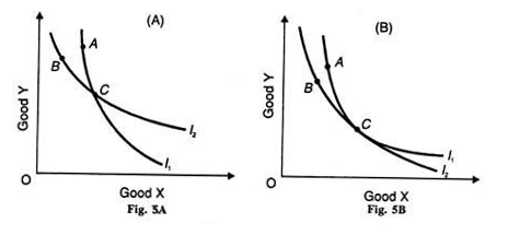
5. Indifference curves can neither touch nor intersect each other so that one indifference curve passes through only one point on an indifference map. What absurdity follows from such a situation can be shown with the help of Figure 5 (A) where the two curves 1₁ and I₂ cut each other.

Point A on the I₂ curve indicates a higher level of satisfaction than point В on the 1₂ curve, as it lies farther away from the origin. But point С which lies on both the curves yields the same level of satisfaction as point A and B.

Thus on the curve I₁: A=C

and on the curve I₂:B=C

A = B

.^..

This is absurd because A is preferred to B, being on a higher indifference curve l₁ Since each indifference curve represents a different level of satisfaction, indifference curves can never intersect at any point. The same reasoning applies if two indifference curves touch each other at point С in Panel (B) of the figure.

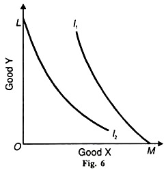
6. An indifference curve cannot touch either axis. If it touches X-axis, as I₂ in Figure 6 at U, the consumer will be having OM quantity of good X and none of Y. Similarly, if an indifference curve I touch the f-axis at L, the consumer will have only OL of Y good and no amount of X. Such curves are in contradiction to the assumption that the consumer buys two goods in combinations.

7. An indifference curve is convex to the origin. The convexity rule implies that as the consumer substitutes X for Y, the marginal rate of substitution diminishes. It means that as the amount X is increased by equal amounts that of Y diminish by smaller amounts.

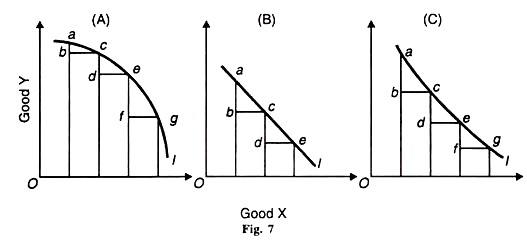
The slope of the curve becomes smaller as we move to the right. To prove this, let us take a concave curve where the marginal rate of substitution of X for Y increases instead of diminishing, i.e., more of У is given up to have additional units of X As in Figure 7 (A), the consumer is giving up ab < cd< ef units of Y for bc = de = fg units of X. But an indifference curve cannot be concave to the origin.

If we take a straight line indifference curve at an angle of 45° with either axis, the marginal rate of substitution between the two goods will be constant, as in Panel (B) where ab of Y= be of X and cd of Y= de of X. Thus an indifference curve cannot be a straight line.

Figure 7(C) shows an indifference curve convex to the origin.

Here the consumer is giving up less and less units of Y in order to have equal additional units of X i.e., ab> cd> ef of Y for bc= de=fg= of X.

Thus an indifference curve is always convex to the origin because the marginal rate of substitution between the two goods declines.

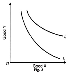
8. Indifference curves are not necessarily parallel to each other. Though they are falling, negatively inclined to the right, yet the rate of fall will not be the same for all indifference curves. In other words, the diminishing marginal rate of substitution between the two goods is essentially not the same in the case of all indifference schedules. The two curves 1_; and I₂ shown in Figure 8 are not parallel to each other.

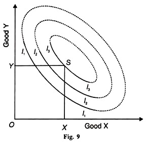
9. In reality, indifference curves are like bangles. But as a matter of principle, their ‘effective region’ in the form of segments is shown in Figure 9. This is so because indifference curves are assumed to be negatively sloping and convex to the origin.

An individual can move to the higher indifference curves I₂ and I₃ until he reaches the saturation point S where his total utility is the maximum. If the consumer increases his consumption beyond X or Y, total utility will fall. If he increases his consumption of X so as to reach the dotted portion of the I₃ curve (horizontally from point S), he gets negative utility.

If to compensate himself for this loss of utility, he increases the consumption of Y, he may be again on the dotted portion of the curve (vertically from point S). Thus the consumer may be on the concave portion of the circular curve. Since by moving to the dotted portion he gets negative utility, the effective region of the circular curve will be the convex portion.