Inflation and Unemployment: Philips Curve and Rational Expectations Theory

Inflation and Unemployment: Philips Curve and Rational Expectations Theory!

Introduction:

In the simple Keynesian model of an economy, the aggregate supply curve (with variable price level) is of inverse L-shape, that is, it is a horizontal straight line up to the full-employment level of output and beyond that it becomes horizontal.

This means that during recession or depression when the economy is having a good deal of excess capacity and large-scale unemployment of labour and idle capital stock, the aggregate supply curve is perfectly elastic.

When full-employment level of output is reached, aggregate supply curve becomes perfectly inelastic. With this shape of aggregate supply curve assumed in the simple Keynesian model, increase in aggregate demand before the level of full employment causes increase in the level of real national output and employment with price level remaining unchanged.

That is, no cost has to be incurred in the form of rise in the price level (i.e., inflation rate) for raising the level of output and reducing unemployment. In the Keynesian model, once the full-employment level of output is reached and aggregate supply curve becomes vertical, further increase in aggregate demand caused by the expansionary fiscal and monetary policies will only raise the price level in the economy.

That is, in this simple Keynesian model, inflation occurs in the economy only after full-employment level of output has been attained. Thus, in the simple Keynesian model with inverse L-shaped aggregate supply curve there is no trade-off or clash between inflation and unemployment.

Inflation-Unemployment Trade-Off: Phillips Curve:

However, the actual empirical evidence did not fit well in the above simple Keynesian macro model. A noted British economist, A.W. Phillips, published an article in 1958 based on his good deal of research using historical data from the U.K. for about 100 years in which he arrived at the conclusion that there in fact existed an inverse relationship between rate of unemployment and rate of inflation.

This inverse relation implies a trade-off, that is, for reducing unemployment, price in the form of a higher rate of inflation has to be paid, and for reducing the rate of inflation, price in terms of a higher rate of unemployment has to be borne.

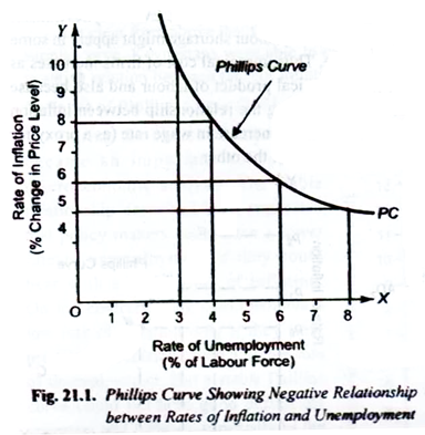
On graphically fitting a curve to the historical data Phillips obtained a downward sloping curve exhibiting the inverse relation between rate of inflation and the rate of unemployment and this curve is now named after his name as Phillips Curve. This Phillips curve is shown in Fig. 21.1 where along the horizontal axis the rate of unemployment and along the vertical axis the rate of inflation is measured.

It will be seen that when rate of inflation is 10 per cent, the unemployment rate is 3 per cent, and when rate of inflation is reduced to 5 per cent per annum, say by pursuing contractionary fiscal policy and thereby reducing aggregate demand, the rate of unemployment increases to 8 per cent of labour force.

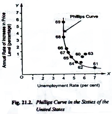
The actual Phillips curve drawn from the data of sixties (1961 -69) for the United States also shows the inverse relation between unemployment rate and rate of inflation (see Fig. 21.2). Such empirical data pertaining to the fifties and sixties for other developed countries seemed to confirm the Phillips curve concept.

On the basis of this, many economists came to believe that there existed a stable Phillips curve which depicted a predictable inverse relation between inflation and unemployment. Further, on the basis of a stable Phillips curve for a country, they emphasized the trade-off that confronts the economic policy makers.

This trade-off presents a dilemma for the policy makers; should they choose a higher rate of inflation with lower unemployment or a higher rate of unemployment with a low inflation rate? In what follows we first explain the rationale underlying the Phillips curve, that is, how the inverse relationship between inflation and unemployment can be theoretically explained.

We will further explain why this concept of stable Phillips curve depicting inverse relation between inflation and unemployment broke down during seventies and early eighties. During seventies a strange phenomenon was witnessed in the USA and Britain when there existed a high rate of inflation side by side with high unemployment rate.

This was contrary to both Phillips curve concept and the simple Keynesian model. This simultaneous existence of both high rate of inflation and high unemployment rate (or low level of real national product) during the seventies and early eighties has been described as stagflation.

Explanation of Phillips Curve:

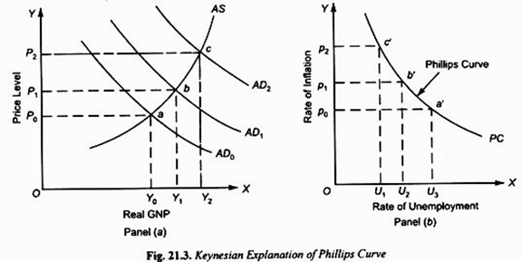
Let us first provide an explanation for the Phillips curve. Both Keynesians and Monetarists agreed to the existence of the Phillips curve. The explanation of Phillips curve by the Keynesian economists is quite simple and is graphically illustrated in Fig. 21.3. It may be noted that Keynesian economists assume the upward-sloping aggregate supply curve.

In fact, Keynes himself recognized that the curve AS is upward sloping in intermediate range, that is, as the economy approaches near-full employment level, the aggregate supply curve slopes upward. According to Keynesian economists, aggregate supply curve is upward sloping for two reasons.

First, as output is increased by the firms in the economy, diminishing returns to variable factors, especially to labour, occur or accrue resulting in fall in marginal physical product (MPP_L) of labour. With money wage rate (W) as given and fixed, the fall in the marginal physical product of labour causes the rise in the marginal cost (MC) of production (Note that MC = W/MPP_L). With the fail in the MPP of labour, wage rate remaining constant, the term W/MPP_L measuring marginal cost (MC) will rise.

The second reason for the marginal cost to go up is the rise in the wage rate as employment and output are increased. When under pressure of aggregate demand for output, demand for labour increases, its wage rate tend to rise, supply curve of labour being upward sloping.

Even Keynes himself believed that as the economy approached near-full employment, labour shortage might appear in some sectors of the economy causing increase in the wage rate. Thus, marginal cost of firms increases as more labour is employed due to diminishing marginal physical product of labour and also because wage rate also rises.

In fact Phillips himself, while discussing the relationship between inflation and unemployment, considered the relationship between rate of increase in wage rate (as a proxy for the rate of inflation) on the one hand and unemployment rate on the other.

Now, it will be seen from panel (a) of Fig. 21.3 that with the initial aggregate demand curve AD₀ and the given aggregate supply curve AS, the price level P₀ and output level Y₀ are determined. Now, suppose the aggregate demand curve increases from AD₀ to AD₁, it will be seen that price level rises to P₁ and aggregate national output increases from Y₀ to Y₁.

Note that increase in aggregate national product means increase in employment of labour and therefore reduction in unemployment rate. Thus the rise in the price level from P₀ to P₁ (i.e., occurrence of inflation) results in lowering of unemployment rate showing inverse relation between the two. Further, if aggregate demand increases to AD₂, the price level further rises to P₂ and national output increases to Y₂ which will further lower the rate of unemployment.

The greater the rate at which aggregate demand increases, the higher will be the rate of inflation which will cause greater increase in aggregate output and employment resulting in much lower rate of unemployment. Thus, a higher rate of increase in aggregate demand and consequently a higher rate of rise in price level is associated with the lower rate of unemployment and vice versa. This is what is represented by Phillips curve.

Consider panel (b) of Fig. 21.3 where point a’ on the downward sloping Phillips curve PC corresponds to point a of panel (a) of Fig. 21.3. In panel (b) of the Fig. 21.3 we have shown the rate of unemployment equal to U₃ corresponding to the price level P₀ of panel (a). When the aggregate demand shifts to AD₁, there is a certain rate of inflation and price level rises to P₁ and aggregate output expands to Y₁.

As seen above, this increase in aggregate output leads to the increase in employment of labour bringing about decline in unemployment rate. Suppose the rate of rise in the price level (i.e., the rate of inflation) when it increases from P₀ to P₁ in panel (a) following the increase in aggregate demand is greater than the rate of rise in the price level of the previous period, we obtain a lower rate of unemployment U₂ than before corresponding to a higher inflation rate p₁ in the Phillips curve PC in panel (b).

With a still higher rate of inflation, say p₂, when price level rises from P₁ to P₂ in panel (a) following the increase in aggregate demand to AD₂, we have a further lower rate of unemployment equal to U₁ in panel (b) corresponding to point c’ on the Phillips curve PC. This gives us a downward-sloping Phillips curve PC.

It is clear from above that through increase in aggregate demand and upward-sloping aggregate supply curve; Keynesians were able to explain the downward-sloping Phillips curve showing the negative relation between rates of inflation and unemployment.

Collapse of Phillips Curve (1971-91):

During the sixties Phillips curve became an important concept of macroeconomic analysis. The stable relationship described by it suggested that policy makers could have a lower rate of unemployment if they could bear with a higher rate of inflation. On the contrary, they could achieve a low rate of inflation only if they were prepared to reconcile with a higher rate of unemployment.

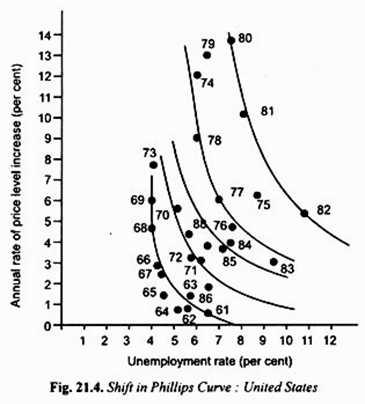
But a stable Phillips curve could not hold good during the o seventies and eighties, especially in the United States. Therefore, experience in the two decades (1971 -91) has prompted some economists to say that the stable Phillips curve has disappeared. Figure 21.4 shows data regarding the behaviour of inflation and unemployment during the seventies and eighties in the United States which do not conform to a stable Phillips curve.

In these two decades we have periods when rates of both inflation and unemployment increased (that is, a high rate of inflation was associated with a high unemployment rate, which shows the absence of trade-off. We have shown the data of inflation rate and unemployment in case of the United States in Fig. 21.4. From the data it appears that instead of remaining stable, the Phillips curve shifted to the right in the seventies and early eighties and to the left during the late eighties, (see Fig. 21.4).

Causes of Shift in Phillips Curve:

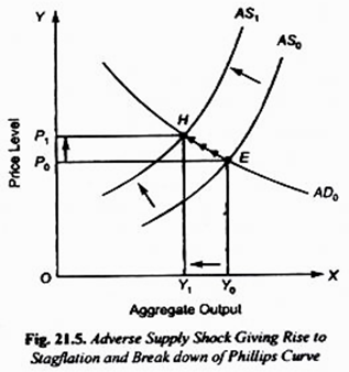
Now, what could be the cause of shift in the Phillips curve? There are two explanations for this. First, according to Keynesians, the occurrence of higher inflation rate along with the increase in unemployment rate witnessed during the seventies and early eighties was due to the adverse supply shocks in the form of fourfold increase in the prices of oil and petroleum products delivered to the American economy first in 1973-74 and then again in 1979-80.

Consider Fig. 21.5 where AD₀ and AS₀ are in equilibrium at point E and determine price level OP₀ and aggregate national output OY₀. The hike in price of oil by OPEC, the cartel of oil producing Middle East countries brought about a rise in the cost of production of several commodities for the production of which oil was used as an energy input. Further, the oil price hike also raised the transportation costs of all commodities.

The increase in cost of production and transportation of commodities caused a shift in the aggregate supply curve upward to the left. This is generally described as adverse supply shock which raised the unit cost at each level of output. It will be seen from Fig. 21.5 that due to this adverse supply shock aggregate supply curve has shifted to the left to the new position AS₁ which intersects the given aggregate demand curve AD₀ at point H.

At the new equilibrium point H, price level has risen to P₁ and output has fallen to OY₁ which will cause unemployment rate to rise. Thus, we have a higher price level with a higher unemployment rate. This explains the rise in the price level with the rise in the unemployment rate, the phenomenon which was witnessed during the seventies and early eighties in the developed capitalist countries such as the U.S.A. Note that this has been interpreted by some economists as a shift in the Phillips curve and some as demise or collapse of the Phillips curve.

Natural Rate Hypothesis and Adaptive Expectations: Friedman’s Views Regarding Phillips Curve:

A second explanation of occurrence of a higher rate of inflation simultaneously with a higher rate of unemployment was provided by Friedman. He challenged the concept of a stable downward- sloping Phillips curve. According to him, though there is a trade-off between rate of inflation and unemployment in the short run, that is, there exists a short-run downward sloping Phillips curve, but it is not stable and it often shifts both leftward and rightward.

He argued that there is no long-run stable trade-off between rates of inflation and unemployment. His view is that the economy is stable in the long run at the natural rate of unemployment and therefore the long-run Phillips curve is a vertical straight line. He argues that misguided Keynesian expansionary fiscal and monetary policies based on the wrong assumption that a stable Phillips curve exists only result in increasing rate of inflation.

Natural Rate of Unemployment:

It is necessary to explain the concept of natural rate of unemployment on which the concept of long-run Phillips curve is based. The natural rate of unemployment is the rate at which in the labour market the current number of unemployed is equal to the number of jobs available. These unemployed workers are unemployed for the frictional and structural reasons, though the equivalent number of jobs is available for them.

For instance, the fresh entrants may spend a good deal of time in searching for the jobs before they are able to find work. Further, some industries may be registering a decline in their production rendering some workers unemployed, while others may be growing creating new jobs for workers.

But the unemployed workers may have to be provided new training and skills before they are deployed in the newly created jobs in the growing industries. It is these frictional and structural unemployment’s that constitute the natural rate of unemployment.

Since the equivalent number of jobs is available for them, full employment is said to prevail even in the presence of this natural rate of unemployment. It is presently believed that 4 to 5 per cent rate of unemployment represents a natural rate of unemployment in the developed countries.

Theory of Adaptive Expectations and Natural Rate Hypothesis:

Another important thing to understand from Friedman’s explanation of shift in the short-run Phillips curve is that expectations about the future rate of inflation play an important role in it. Friedman put forward a theory of adaptive expectations according to which people from their expectations on the basis of previous and present rate of inflation, and change or adapt their expectations only when the actual inflation turns out to be different from their expected rate.

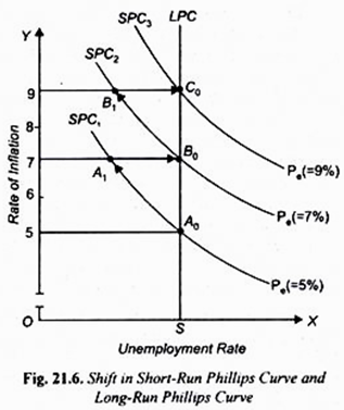
According to this Friedman’s theory of adaptive expectations, there may be a trade-off between rates of inflation and unemployment in the short run, but there is no such trade-off in the long run. The view of Friedman and his follower monetarists is illustrated in Figure 21.6. To begin with SPC₁ is the short-run Phillips curve and the economy is at point A₀, on it corresponding to the natural rate of unemployment equal to 5 per cent of labour force. The location of this point A₀ on the short-run Phillips curve depends on the level of aggregate demand.

Further, we assume that the economy is currently experiencing a rate of inflation equal to 5%. The other assumption we make is that nominal wages have been set on the expectations that 5 per cent rate of inflation will continue in the future.

Now, suppose for some reasons the government adopts expansionary fiscal and monetary policies to raise aggregate demand. The consequent increase in aggregate demand will cause the rate of inflation to rise, say to seven per cent. Given the level of money wage rate which was fixed on the basis that the 5 per cent rate of inflation would continue to occur, the higher price level than expected would raise the profits of the firms which will induce the firms to increase their output and employ more labour.

As a result of the increase in aggregate demand resulting in a higher rate of inflation and more output and employment, the economy will move to point A₁ on the short- run Phillips curve SPC₁ in Figure 21.6, where unemployment has decreased to 3.5 per cent while inflation rate has risen to 7%.

It may be noted from Figure 21.6 that in moving from point A₀ to A₁, on SPC₁ the economy accepts a higher rate of inflation at the cost of achieving a lower rate of unemployment. Thus, this is in conformity with the concept of Phillips curve explained earlier. However, the advocates of natural rate theory interpret it in a slightly different way.

They think that lower rate of unemployment achieved is only a temporary phenomenon. They think when the actual rate of inflation exceeds the one that is expected, unemployment rate will fall below the natural rate only in the short run. In the long run, the natural rate of unemployment will be restored.

Long-Run Phillips Curve and Adaptive Expectations:

This brings us to the concept of long-run Phillips curve, which Friedman and other natural rate theorists have put forward. According to them, the economy will not remain in a stable equilibrium position at A₁. This is because the workers will realize that due to the higher rate of inflation than the expected one, their real wages and incomes have fallen.

The workers will therefore demand higher nominal wages to restore their real income. But as nominal wages rise to compensate for the higher rate of inflation than expected, profits of business firms will fall to their earlier levels. This reduction in their profit implies that the original motivation that prompted them to expand output and increase employment resulting in lower unemployment rate will no longer be there.

Consequently, they will reduce employment till the unemployment rate rises to the natural level of 5%. That is, with the increase is nominal wages in Figure 21.6 the economy will move from A₁ to B₀, at a higher inflation rate of 7%. It may be noted that the higher level of aggregate demand which generated inflation rate of 7% and caused the economy to shift from A₀ to A₁ still persist.

Further, at point B₀, and with the actual present rate of inflation equal to 7 per cent, the workers will now expect this 7 per cent inflation rate to continue in future. As a result, the short-run Phillips curve SPC shifts upward from SPC₁ to SPC₂. It therefore follows, according to Friedman and other natural rate theorists, that the movement along a Phillips curve SPC is only a temporary or short-run phenomenon.

In the long when nominal wages are fully adjusted to the changes in the inflation rate and consequently unemployment rate comes back to its natural level, a new short-run Phillips curve is formed at the higher expected rate of inflation.

However, the above process of reduction in unemployment rate and then its returning to the natural level may continue further. The Government may misjudge the situation and think that 7 per cent rate of inflation is too high and adopt expansionary fiscal and monetary policies to increase aggregate demand and thereby to expand the level of employment.

With the new increase in aggregate demand, the price level will rise further with nominal wages lagging behind in the short-run. As a result, profits of business firms will increase and they will expand output and employment causing the reduction in rate of unemployment and rise in the inflation rate. With this, the economy will move from B₀ to B₁ along their short-run Phillips curve SPC₂.

After some time, the workers will recognize the fall in their real wages and press for higher normal wages to compensate for the higher rate of inflation than expected. When this higher nominal wages are granted, the business profits decline which will cause the level of employment to fall and unemployment rate to return to the natural rate of 5%. That is, in Figure 21.6 the economy moves from point B₁ to C₀.

The new short-run Phillips curve will now shift to SPC₂ passing through point C₀. The process may be repeated again with the result that while in the short run, the unemployment rate falls below the natural rate, in the long run it returns to its natural rate. But throughout this process the inflation rate continuously goes on rising.

On joining points such as A₀, B₀, C₀ corresponding to the given natural rate of unemployment we get a vertical long-run Phillips curve LPC in Figure 21.6. Thus, in the adaptive expectations theory of the natural rate hypothesis while the short-run Phillips curve is downward sloping indicating that trade­off between inflation and unemployment rate the short run, the long run Phillips curve is a vertical straight line showing that no trade-off exists between inflation and unemployment in the long run.

It is important to remember that adaptive expectations theory has also been applied to explain the reverse process of disinflation, that is, fall in the rate of inflation as well as inflation itself. Suppose in Figure 21.6 the economy is originally at point C₀ with 9% rate of inflation.

Now, if a decline in aggregate demand occurs, say as a result of contraction of money supply by the Central Bank of a country, this will reduce inflation rate below the 9 per cent expected rate. As a result, profits of business firms will decline because the prices will be falling more rapidly than wages. The decline in profits will cause the firms to reduce employment and consequently unemployment rate will rise.

Eventually, firms and workers will adjust their expectations and the unemployment rate will return to the natural rate. The process will be repeated and the economy in the long run will slide down along the vertical long-run Phillips curve showing falling rate of inflation at the given natural rate of unemployment.

It follows from above that according to adaptive expectations theory any rate of inflation can occur in the long run with the natural rate of unemployment.

Long-Rung Phillips Curve: Rational Expectations Theory:

In the end we explain the viewpoint about inflation and unemployment put forward by Rational Expectations Theory which is the cornerstone of recently developed macroeconomic theory, popularly called new classical macroeconomics. Friedman’s adaptive expectations theory assumes that nominal wages lag behind changes in the price level.

This lag in the adjustment of nominal wages to the price level brings about rise in business profits which induces the firms to expand output and employment in the short run and leads to the reduction in unemployment rate below the natural rate. According to the rational expectations theory, which is another version of natural unemployment rate theory, there is no lag in the adjustment of nominal wages consequent to the rise in price level.

The advocates of this theory further argue that nominal wages are quickly adjusted to any expected changes in the price level so that there does not exist Phillips curve showing trade-off between rates of inflation and unemployment. According to them, as a result of increase in aggregate demand, there is no reduction in unemployment rate.

The rate of inflation resulting from increase in aggregate demand is fully and correctly anticipated by workers and business firms and get completely and quickly incorporated into the wage agreements resulting in higher prices of products.

Thus, it is the price level that rises, the level of real output and employment remaining unchanged at the natural level. Hence, aggregate supply curve according to the rational expectations theory is a vertical straight line at the full-employment level.

Rational expectations theory rests on two basic elements. First, according to it, workers and producers being quite rational have a correct understanding of the economy and therefore correctly anticipate the effects of the Government’s economic policies using all the available relevant information. On the basis of these anticipations of the effects of economic events and Government’s policies they take correct decisions to promote their own interests.

The second premise of rational expectations theory is that, like the classical economists, it assumes that all product and factor markets are highly competitive. As a result, wages and product prices are highly flexible and therefore can quickly change upward and downward.

Indeed, the rational expectations theory considers that new information is quickly assimilated (i.e., taken into account) in the demand and supply curves of markets so that new equilibrium prices immediately adjust to the new economic events and policies, be it a new technological change or a supply shock such as a drought or act of OPEC oil cartel or change in Government’s monetary and fiscal policies.

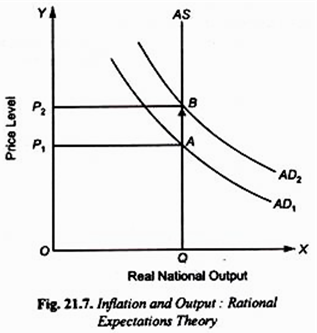
Figure 21.7 illustrates the standpoint of rational expectations theory about the relation between inflation and unemployment. In this OQ is the level of real national output corresponding to the full employment of labour (with a given natural rate of unemployment). AS is aggregate supply curve at OQ level of real national output.

To begin with, AD₁ is the aggregate demand curve which intersects the aggregate supply curve AS at point A and determines price level equal to P₁. Suppose Government adopts an expansionary monetary policy to increase output and employment. As a consequence, aggregate demand curve shifts upward to the new position AD₂.

According to rational expectations theory, people (i.e., workers, businessmen, consumers, lenders) will correctly anticipate that this expansionary policy will cause inflation in the economy and they would take prompt measures to protect themselves against this inflation. Accordingly, workers would press for higher wages and get it granted, businessmen would raise the prices of their products, lenders would hike their rates of interest.

All these increases would take place immediately. It is thus clear that the increase in aggregate demand (i.e., aggregate expenditure) brought about by expansionary monetary policy will cause the price level to rise to P₂. Thus, the increase in aggregate demand or expenditure will be fully reflected in higher wages, higher interest rates and higher product prices, all of which will rise in proportion to the anticipated rate of inflation.

Consequently, the levels of real national product and employment, wage rate, interest rate, levels of investment and consumption would remain unchanged. This can be easily understood with the help of monetarist equation of exchange P = MV/Q. Expansionary monetary policy leads to the increase in money supply M.

As a result, aggregate expenditure, which in quantity theory, is equal to MV increases. (Note that V is the velocity of circulation of money which remains stable). But people’s anticipations or expectations of inflation cause an increase in P in equal proportion to the expansion in MV. This means that despite the increase in MV, real output Q and the level of employment will remain unchanged.

It is clear from above that people’s anticipations or expectations of inflation and acting upon them in their decision making when expansionary monetary policy is adopted frustrate or nullify the intended effect (that is, increase in real output and employment) of Government’s monetary policy.

In other words, according to the rational expectations theory, the intended effect of expansionary monetary policy on investment, real output and employment does not materialize. As seen above, in Fig. 21.7 it is due to the anticipation of inflation by the people and quick upward adjustments made in wages, interest etc., by them that the price level instantly rises from P₁ to P₂, the level of output Q remaining constant.

That is why, according to the rational expectations theory, aggregate supply curve is a vertical straight line. The vertical aggregate supply curve means that there is no trade­off between inflation and unemployment, that is, downward-sloping Phillips curve does not exist. Thus, according to rational expectations theory, the increase in aggregate demand or expenditure as a consequence of easy monetary policy of the Government will fail to reduce unemployment and instead will only cause inflation in the economy.