Input-Output Analysis in Economics | Economics

One of the most interesting developments in the field of modern economics is the model of industrial interdependence known as input-output tableau. It owes its origin to Prof. Wassily Leontief. Input-output analysis is of special interest to the national-income economist because it provides a very detailed breakdown of the macro-aggregates and money flows. This model is widely used in planning and forecasting.

Input-Output Flow Tables:

Leontief imagines an economy in which goods like iron, coal, alcohol, etc. are produced in their respective industries by means of a primary factor, viz., labour, and by means of other inputs such as iron, coal, alcohol, etc. For the production of iron, coal is required.

A Two-Industry Example:

Let us imagine, following Leontief, a simple economy in which there are two industries—agriculture and manufacturing. Each directly requires the use of a primary factor called labour in its production process, and each requires in its productive process inputs which are output of the other industry.

Table 1 provides a simplified picture of such an economy. Agriculture and manufacturing are the first two entries, and each of their rows will show what happens to their total output. The third row is given to the primary factor, labour, of which the community has a total of 50 units (thousands of man-years) per year. These 50 units of labour are allocated as inputs to the two industries in the respective amounts 10 and 40.

The first row total shows that the agricultural output totals 250 units (million of tons) per year. Of this total, 50 units go directly to final consumption, i.e., to households and government, as shown in the third column of row 1. What happens to the remaining 200 units of agricultural output?

They are required as inputs to help make possible the community’s production of manufactured and agricultural goods. Thus 175 units of agricultural output is required as material inputs in order to make possible manufacturing production: this is shown in the second column of the first row.

The remainder of agricultural output, 25 units, is required in agriculture itself, e.g., that used to feed cows that turn out wheat, and is shown in column 1 of row h Similarly, row 2 shows the allocation of the total output of manufacturing industries, 120 units (thousand of dozens) per year, among final consumption and intermediate inputs needed in two industries.

In row 2, columns 1, 2 and 3 show allocations of 40, 20 and 60 units of manufactured goods per year to agriculture manufacturing and final consumption (households and governments). All the items in Table 1 are flows, i.e., physical units to per year (and not stocks like capital or intangibles).

The ‘total outputs’ column gives the overall input of labour and output of each commodity. The first column describes the input or cost structure of the agricultural industry : the 250-unit agricultural output was produced with the use of 25 units of agricultural goods, 40 units of manufacturing goods, and 10 units of labour.

Similarly, the second column details the observed input structure of the manufacturing industry. The ‘final demand’ column shows the commodity breakdown of what is available for consumption and government expenditure. Labour is assumed not to be directly consumed.

Suppose, however, that we had deliberately chosen the physical units in which each commodity is measured so that at some given base prices, one unit costs Re. 1. Then each entry in Table 1 becomes a rupee value and the columns can be measured virtually (literally) as cost figures. If we add down the columns, the sum gives the total cost of producing the industry’s output.

Since the output is also measured in terms of rupee values, total output is the same as total revenue. Thus agricultural revenue (at the base prices) is Rs 250 million, and cost of production is Rs 75 mn. In manufacturing, revenue is Rs 120 mn, and cost Rs 235 mn. Thus in agriculture there was a profit of Rs 175 million, and in manufacturing there was a loss of Rs 115 mn.

These items in Table 1 show that the sales of the two industries to themselves and to each other might be described as “non-GNP” items. The ‘final demand’ column represents the output side of GNP, and the labour row represents the factor-cost side.

The economy can be thought of as a machine that uses up labour (and has 50 units of labour per year at its disposal) and produces final consumption. With its 50 units of labour the economy is capable of producing an annual flow of 50 units of agricultural goods and 60 units of manufactures.

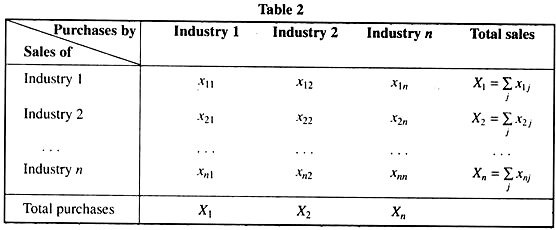
In Table 2 the sum of the rows shows the total value that has been sold or allocated to consumption and all industrial uses. The sum of any column is the same as the sum of the corresponding row. In its ‘static’ version, Leontief’s input-output analysis deals with a particular question- what level of output should each of the industries in an economy produce, in order that it will just be sufficient to satisfy the total demand for the product?

The rationale for the term input-output is quite plain to see. The output of any industry (say, the steel industry) is needed as an input in many other industries, or even for that industry itself; therefore, the ‘correct’ level of steel output will depend on the input requirements of all the n industries.

In turn, the output of many other industries will enter into the steel industry as inputs and, consequently, the ‘correct’ levels of other products will depend partly upon the input requirements of the steel industry. In view of this inter-industry dependence, any set of ‘correct’ output levels for the n industries must be one that is consistent with all the input requirements in the economy, so that no bottlenecks can arise anywhere.

In this light, it is clear that input-output analysis should be of great use in production planning, such as in planning for the economic development of a country or for a programme of national defence.

Let us assume:

(i) Each industry produces only one homogeneous commodity. (Broadly interpreted, this does permit the case of two or more jointly produced commodities, provided they are produced in a fixed proportion to one another.)

(ii) Each industry uses a fixed input ratio (or factor combination) for the production of its output.

(iii) Production in every industry is subject to constant returns to scale so that a k-fold change in every input will result in an exactly k-fold change in the output.

In order to produce each unit of the j-th commodity, the input need for the i-th commodity must be a fixed amount, which we shall denote by a_1j. Specifically, the production of each unit of the j-th commodity will require a_1j (amount) of the first commodity, a_2j of the second commodity,…., and a_nj of the nth commodity. (The first subscript refers to the input, and the second to the output, so that a_1j indicates how much of the i-th commodity is used for the production of each unit of the j-th commodity.) We may also assume prices to be given and, thus, adopt “a rupee’s worth” of each commodity as its unit.

Then the statement a₂₂ = 0.35 will mean that 35 paise’s worth of the third commodity is required as an input for producing a rupee’s worth of the second commodity. The a_1j symbol is referred to as an input coefficient.

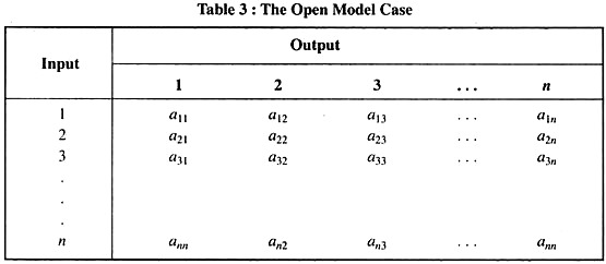
For an n-industry economy, the input coefficient can be arranged into a matrix A = [a_1j] as in Table 3, in which each column specifies the input requirements for the production of one unit of the output of a particular industry.

The second column, for example, states that to produce a unit (a rupee’s worth) of commodity 2, the inputs required are- a₁₂ units of commodity 1, a₂₂ units of commodity 2, etc. If no industry uses its own product as an input, then the elements in the principal diagonal of matrix A will be all zero.

The Open Model:

If, besides the n industries, the model contains an “open” sector (say, households) which exogenously determines a final demand (non-input demand) for the product of each industry and which supplies a primary input (say, labour service) not produced by the n industries themselves, then the model is an open one (Table 3).

In view of the presence of the open sector, the sum of the elements in each column of the input-coefficient matrix A (or input matrix A, for short) must be less than 1. Each column sum represents the partial input cost (not including the cost of the primary input) incurred in producing a rupee’s worth of some commodity; if this sum is greater than Re. 1, production will not be economically justifiable. Symbolically, this fact may be stated thus:

Carrying this line of thought a step further, it may also be stated that, since the value of output (Re. 1) must be fully absorbed by the payment to all factors of production, the amount by which the column sum falls short of Re. 1 must represent the payment to the primary input (labour here) of the open sector. Thus the value of the primary input needed in producing a unit of the j-th commodity should be

If industry 1 is to produce an output just sufficient to meet the input requirements of the n industries as well as the final demand of the open sector, its output level x₁ must satisfy the following equation:

where d₁ denotes the final demand for its output and a_1j x_j represents the input requirement of the j-th industry.

The equation may also be written as:

Note that aside from the first coefficient, (1 – α₁₁), the remaining coefficients in the above equation can be transplanted directly from the first row of Table 3, except that they are now prefixed with minus signs.

Similarly, the corresponding equation for industry 2 will have the same coefficients as in the second row of Table 3 (again with minus signs added), except that the variable x₂ will have the coefficient (1 – α₂₂).

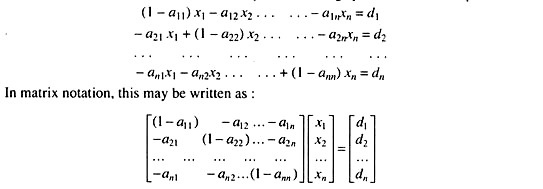
For the entire set of n industries, the ‘correct’ output levels can, therefore, be summarised by the following system of n linear equations:

If the 1 ‘s in the principal diagonal of the matrix are ignored, the new matrix is simply -A = [- a_1j], As it is, on the other hand, the matrix is the sum of the identity matrix I_n (with 1 ‘s in its principal diagonal and with O’s everywhere else) and the matrix – A. Thus the above matrix can also be written

(I-A) x = d

where x and d are, respectively, the output vector and the final demand (constant-term) vector. The matrix (I-A) is called the technology matrix. If (I-A) is non-singular — and there is no a priori reason why it should not be — then the inverse (I-A) can be found, and the system will have the unique solution-

x = (I-A)^-1 d

The Closed Model:

If the exogenous sector of the open input-output model is absorbed into the system as just another industry, the model will become a closed one. In such a model, final demand and primary input do not appear; in their place will be the input requirements and the output of the newly conceived industry. All goods will now be intermediate in nature, because everything is produced only for the sake of satisfying the input requirements of the (n + 1) sectors in the model.

At first glance, the conversion of the open sector into an additional industry would not seem to create any significant change in the analysis. Actually, however, since the new industry is assumed to have a fixed input requirement it must now bear a fixed proportion to the labour service they supply. This constitutes a significant change in the analytical framework of the model.

Mathematically, the disappearance of the final demands means that we will now have a homogeneous equation system.

Assuming four industries only (including the new one, designated by the 0 subscript), the ‘correct’ output levels will be, by analogy of the above matrix, those which satisfy the following equation systems:

Being homogeneous, this equation system can have a non-trivial solution if and only if the 4 x 4 technology matrix (I – A) has a vanishing determinant. The latter condition is indeed always fulfilled : In a closed model, there is no more primary input; hence the column sum in the input-coefficient matrix A must now be exactly equal to (rather than less than) l; that is

a_0j + a_1j + a_2j + a_3j = 1

or a_0j = 1 – a_1j – a_2j – a_3j

But this implies that, in every column of the matrix (I-A) above, the top element is always equal to the negative of the sum of the other three elements. Consequently, the four rows are linearly dependent, and we must find |I -A| = 0. This guarantees that the system does possess non-trivial solutions; in fact, it has an infinite number of them.

This means that in a closed model, with a homogeneous-linear equation system, no unique ‘correct’ output mix exists. We can determine the output levels x₁……………….. x₃ in proportion to one another, but cannot fix their absolute levels unless additional restrictions are imposed on the model.

Mathematical Interpretation:

The simple input-output model can well be presented in terms of a few mathematical equations and symbols and on the basis of certain technological assumptions.

If we call agriculture industry 1, manufacturing industry 2 and give labour the subscript 0, then the previous table can be presented as:

since X₁ and X₂ are the total outputs. In addition, we can always add across the rows, so we know that

Leontief assumes:

1. There exist constant returns to scale.

2. There exists fixed coefficients of production, i.e., he supposes that it takes a certain minimal input of each commodity per unit of output of each commodity. The word “minimal” is of some importance- if it takes 2 tonnes of iron ore to produce 1 tonne of iron, no doubt the same iron could be produced from even more ore, but as long as iron has value, nobody will be silly enough to use more than the absolutely required 2 tonnes.

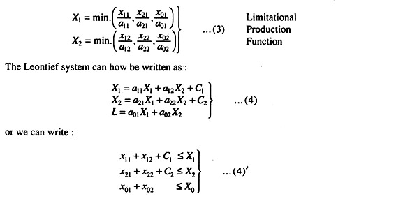
This special Leontief production function can be written in the usual form (1). Let a_1j be the required minimal input of commodity i per unit of output of commodity j (here i = 0, 1, or 2, and j = 1 or 2). Then

The available output certainly cannot be less than the sum of its alternative uses, but it could, physically, be greater.

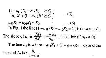
We can account for the output X₁ as follows; a₁₁X₁ will be used up in industry 1 itself, and a₁₂X₂ in industry 2. What is left will be used up for final consumption C₁, viz.,

C₁= X₁-a₁₁X₁ – a₁₂X₂

Similarly for X₂, i.e., C₂ = X₂ – a₂₁X_x – a₂₂X₂. Labour is not produced but is available in amounts up to X₀; the use of labour is a₀₁X₁ in industry 1 and a₀₂X₂ in industry 2.

Thus we get:

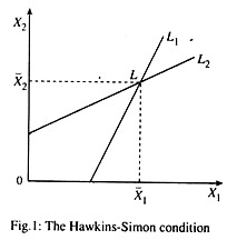
L₁and L₂ intersect at L. If L₁ and L₂ were parallel, i.e., if they had equal slopes, there would be no such point as 1. Any gross-output levels in this region will enable society to consume C₁ and C₂ of the two commodities. In fact, if L₂ had a bigger slope than L₁ there would also be no point L. What is the condition that L should exist or that some bill of goods should be producible? It is that the slope of L₂ must be less than the slope of L₁ i.e.,

As we earlier required that we should not take a direct input of more than one ton of coal to make one tonne of coal, inequalities (7) or (8) assure us that if we add up the direct and indirect inputs of coal that go into a ton of output (coal to make coal) that this will be less than one tonne.

Clearly if a tonne of coal “contains”, directly and indirectly, more than a ton of coal, self-contained production is not viable. If a technology is to be viable at all, each of the “own” input coefficients, a₁₁ and a₂₂ must be less than unity. Otherwise, there would be negative net outputs (1 – a₁₁ and 1 – a₂₂).

The inequality (7) together with earlier 1 – a₁₁ > 0 and 1 – a₂₂ > 0 comprise what are called the Hawkins-Simon conditions.

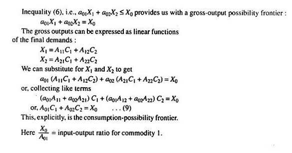
Multiply the first equation in (4) above by 1 – a₂₂, the second by a₂₂ and add to get

Now A₀₁ is the direct labour input not into a unit of C₁ but into the gross direct and indirect X₁ and X₂ needed to support a unit of C₁. In other words, A₀₁ represents the total direct and indirect labour embodied in a unit of final consumption of commodity and A₀₂ is the same for a unit of final consumption of commodity 2. The schedule in (9) simply says that only those bill of final demand are producible and efficient which require X₀ units of labour to support them.

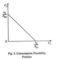
A consumption possibility schedule (9), drawn in Fig. 2, can be thought of as a social transformation curve. If it is desired to consume only C₁an amount X₀/A₀₁ can be produced, given the available resources and technology.

If it is desired to give up some C₁in favour of C₂, such substitutions are possible along the transformation curve. Because the frontier is a straight line, substitution of C₂ for C₁ takes place at constant costs. The MRS is constant, viz.,

Giving up one unit of C₁ sets free (directly and indirectly) A₀i units of labour. To get 1 more unit of C₂ requires A₀₂ units of labour. By giving up 1 unit of C₁ society can, therefore, procure for itself A₀₁/A₀₂ units of C₂. The straight line constant cost nature of the transformation curve reflects not only the linearity of the technology, but also the presence of only one primary factor and the absence of joint production.

Prices in the Leontief Model:

The constant MRS was shown to be A₀₁/ A₀₂. This must determine the relative price of the two commodities:

We have interpreted A₀i as the total labour content of 1 unit of final output of commodity 1. If we designate the wage rate by W, this tells us that

since labour is the only cost-generating element in the system. A real system like Leontief’s can only hope to determine relative prices. The absolute level of prices remains completely indeterminate.