According to the modern theory, there are four determinants of the rate of interest:
(a) The saving function,
(b) The investment function,
(c) Liquidity preference function and
ADVERTISEMENTS:
(d) The quantity of money.
The equilibrium between these four variables together determines the rate of interest as well as the equilibrium level of income. According to Hansen, “An equilibrium condition is reached, when the desired volume of cash balances equals the quantity of money, when the marginal efficiency of capital is equal to the rate of interest and finally, when the volume of investment is equal to the normal or desired volume of saving. And these factors are integrated.
The main weakness of the other theories of interest is that they assume the level of income as constant and do not take into consideration its influence on the rate of interest. The loanable funds theory does not tell us what the rate of interest will be, but gives us the IS curve. IS curve is a negatively sloping curve showing different levels of income at different rates of interest.
Similarly, the liquidity preference theory does not tell the rate of interest, but supplies only the LM curve. LM curve is a positively sloping curve showing different rates of interest at different levels of income. While, IS curve depicts the relationship between the rate of interest and income as determined by the equality of saving and investment, LM curve gives the relationship between the rate of interest and income as determined by the equality of demand and supply of money.
ADVERTISEMENTS:
The loanable funds theory provides a family of saving curves at different levels of income. These together with the investment demand curve give the IS curve. It is a well-known fact that investment is a decreasing function of the rate of interest (i.e., at high interest rate, the investment is low and vice versa) and the saving is an increasing function of income (i.e., when income increases, saving also increases and vice versa).
Given the investment demand schedule, the family of saving schedules gives different points of equality between saving and investment, indicating different rates of interest corresponding to different levels of income. Thus IS curve shows equilibrium in the real sector (product market), indicating various combinations of income levels and interest rates at which there is equilibrium between aggregate real saving and aggregate real investment.
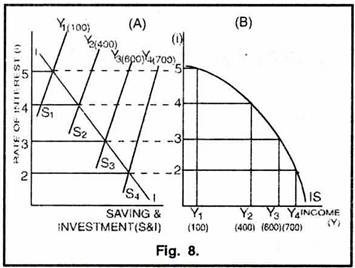
Table 2 and Figure 8 (A& B) explain the derivation of IS curve. In Figure 8 A, let Y1, Y2, Y3 and Y4 represent the income level of Rs. 100, 400, 600, and 700 crores respectively. S1Y1, S2Y2, S3Y3 and S4 Y4 are the saving curves at income levels Y1, Y2, Y3 and Y4 respectively. II is the investment curve. At income level Y1 (100), the equilibrium saving and investment is established at 5% rate of interest. Similarly, at income level Y2 (400), the equilibrium rate of interest is 4%; at income level Y3 (600), the equilibrium rate of interest is 3%; and at income level Y4 (700), the equilibrium rate of interest is 2%. Connecting various equilibrium rates of interest with their corresponding income levels, IS curve is obtained in Figure 8B.
Slope and Shift in IS Curve:
The IS curve slopes downwards to the right. The reason for the negative slope of the IS curve is that at higher levels of income, saving is greater; greater the saving, lower will be the rate of interest; as the rate of interest falls, investment increases till it becomes equal to the higher savings. Thus, as income increases, the equality between saving and investment is established at a lower rate of interest and as income decreases the saving-investment equality is established at the higher rate of interest.
The position of the IS curve depends upon – (a) the saving schedule (or the consumption function) and (b) the investment schedule (or the marginal efficiency of capital). An upward movement in the investment schedule (II curve), or downward movement of the saving schedule (SY curve) or both will raise the level of income corresponding to a given rate of interest.
Consequently, there will be an upward shift in IS curve. In other words, if profit expectations increase or if the people become less thrifty, the IS curve will shift to the right. On the other hand, if profit expectations fall or total consumption expenditure of the community decreases, the IS curve will shift to the left.
Keynes’ liquidity preference theory provides a family of LP schedules at different levels of income. These together with the supply of money curve give the LM curve. The supply of money is fixed by the monetary authority and is interest-inelastic as represented by a vertical line.
Liquidity preference (or demand for holding money in cash) is an increasing function of income implying that as income increases, the liquidity preference also increases and vice versa. Given the supply of money, the family of LP schedules gives different points of equilibrium between liquidity preference and supply of money which indicate different rates of interest corresponding to different levels of income.
Thus, LM curve, which is derived from the family of LP schedules by holding the money supply constant, represents equilibrium in the monetary sector indicating all combinations of income levels and interest rates at which there is equilibrium between the total demand for money (liquidity preference) and the supply of money. The LM curve is the locus of points of equilibrium between the liquidity preference (L) and the supply of money (M), just as the IS curve is the locus of points of equilibrium between investment (I) and saving (S).
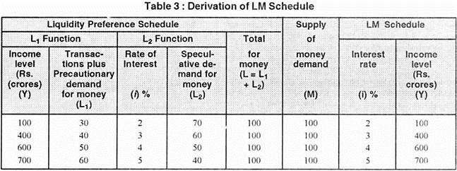
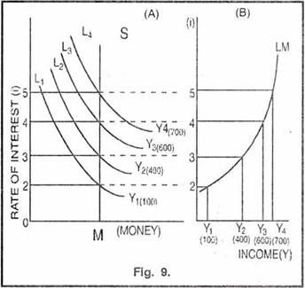
The derivation of LM curve is illustrated in Table 3 and Figure 9 A & B. In Figure 9A, L1 Y1, L2Y2, L3Y3, and L4Y4 are the liquidity preference curves at income levels Y1, Y2, Y3 and Y4 respectively. Y1, Y2, Y3 and Y4 represent the income levels of Rs 100, 400, 600 and 700 cores respectively. SM is the supply of money curve representing fixed money supply OM.
At Y1 (100) income level, the equilibrium between the demand for and supply of money is established at 2% rate of interest. In the same manner, at income level Y2 (400), the equilibrium rate of interest is 3%, at income level Y3 (600), the equilibrium rate of interest is 4%, and at income level Y4 (700), the equilibrium rate of interest is 5%. By relating various equilibrium rates of interest with the corresponding income levels, we get the LM curve as shown in Figure 9B.
Slope of and Shift in LM Curve:
ADVERTISEMENTS:
The LM curve slopes upward to the right for the simple reason that changes in income lead to changes in the rate of interest in the same direction. As income increases, the demand for money (or liquidity preference) increases because of increase in transactions demand for money (L1). Given the fixed supply of money, the quantity of money demanded exceeds the available supply of money.
As a result, people will sell bonds to satisfy their increased liquidity preference, bond prices will fall and the interest rate will rise. Similarly, as income falls, the demand for money decreases because of a decline in transactions demand (L1); there will be excess money supply available for speculative (L2); the money holders-Mil purchase bonds and, as a result, bond prices will increase and the interest rates will fall.
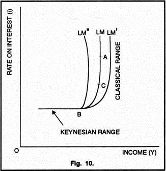
The LM curve becomes highly inelastic at relatively high levels of income (i. e., as the economy moves from point C to point A in Figure 10). At higher income levels, there is larger transactions demand (L1) for fixed money supply and therefore the rate of interest rises steeply. On the other hand, the LM curve becomes steeply elastic at relatively low levels of income (i.e., as the economy moves from point C to B, in Figure 10).
ADVERTISEMENTS:
At lower levels of income, there is smaller transactions demand (L1) for money and so larger part of money supply becomes available for speculative motive (L2) and as a result of this excess money supply, the rate of interest will fall. But since the liquidity preference curve is highly elastic at low interest rates due to speculate demand for money, excess money supply at low levels of income will not reduce interest rates below a certain limit. Thus, LM curve becomes highly interest elastic at low levels of income.
The vertical region (above point A in figure 10) on the LM curve is referred to as the classical range. The classical economists maintained that money was only a medium of exchange and is never held for speculative purposes. In accordance with this thinking, in the classical region of the LM curve, the entire money supply is held for transactions motive (for L1).
Interest rates are so high that bonds become less risky and hence all cash balances kept for speculative motive (for L2) are made available for transactions motive. Or in other words, L2 = 0. Given the money supply (M), the national income (Y) is at its maximum level, and thus velocity of money is also maximum (V = Y/M). In this vertical region of the LM curve, money supply becomes a bottleneck to further expansion of national output.
The horizontal region of the LM curve (to the left of point B in Figure 10) is referred to the Keynesian range because it results from Keynes’ ‘liquidity trap’ hypothesis. In the Keynesian region of the LM curve, the income level (Y), the interest (i), and the velocity of money (V = Y/M) are at the extremely low levels (given the constant money supply (M)), and the people are prepared to hold money in the form of speculative demand for money (L2).
In this horizontal region, very low levels of income reduce the transaction demand for money (L1) but these excess cash balances are not used to purchase bonds ; they are merely held in cash form for speculative motive (i.e., in the form of L2). The reason for this is that because interest rates are so low and the purchase of bonds is so risky that the holders of money balances prefer to hold them rather than to purchase bonds; hence the interest rates will not decline further. Since a lower income level no longer leads to a lower interest rate, the LM curve becomes perfectly elastic, i.e., a horizontal line.
Since LM curve is derived for a constant money supply, changes in the money supply will cause shifts in the LM curve. If the money supply increases the LM curve will shift rightward from LM to LM’ because any given rate of interest is now associated with a higher level of income (except in the Keynesian range). If the money supply falls, the LM curve shifts leftward from LM to LM” because any given rate of interest is now associated with a lower level of income.
ADVERTISEMENTS:
Determination of Rate of Interest:
According to the modern theory of interest, the equilibrium rate of interest and equilibrium level of income are determined simultaneously at the point of intersection between the IS and the LM curves. The IS curve, which represents various combinations of the level of income and the interest rate, denotes equilibrium in the real sector; at each point on the IS curve, saving and investment are equal (S = I).
The LM curve, which also shows various combinations of the income level and the interest rate, denotes equilibrium in the monetary sector; at each point on the LM curve, the demand for money and the supply of money are equal (L = M). Hence, aggregate or general equilibrium (i.e., simultaneous equilibrium in both the money and real markets) will exist at the point of intersection of the IS and LM curves.
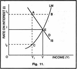
In figure 11, the general equilibrium is reached at point E where IS and LM curves intersect each other. The equilibrium rate of interest is Oi and the equilibrium income level is OY. Oi and OY is the only combination of rate of interest and income at which both real and monetary markets are in equilibrium (i.e., both S = I and L = M). All other combinations of income and rate of interest are disequilibrium combinations.
Consider, for example, point A on IS curve representing the combination of OY1 and Oi1. At point A. the product market is in equilibrium (S = I) since point A is on the IS curve, but the money market is not in equilibrium (M > L). (Since, points A and B are at the same interest rate Oi, and since demand for money (L) equals supply of money (M) at point B, it follows that M > L at point A).
ADVERTISEMENTS:
After meeting the transactions demand (L1) corresponding to the income level OY1, the balance excess money supply (because of M > L) will flow into the bond market, raise the bond prices and cause the interest rate to fail. The fall in the interest rate will increase investment and thus income. This moves the economy down the IS curve towards the equilibrium point E. In the same manner, an opposite disequilibrium represented by point D on IS curve, in which again S = I, but L > M, would be corrected.
Now consider point C on LM curve representing the disequilibrium combination of Y1 and i2. At this point C, the money market is in equilibrium (L = M), since it is on LM curve, but the product market is not in equilibrium, since at Y1 income level, point C indicates excess of investment over saving (I > S). Since, saving equals investment at point A (being on the IS curve) and since the rate of interest is higher at point A than at point C (Oi1 > Oi2), it follows that investment must be greater at point C than at point A.
Thus, at point C, (I > S). Excess of investment will cause output and income to rise. The increase in income leads to an increase in transactions demand for money (L1) which, in turn, raises the rate of interest. This will move the economy up the LM curve towards the equilibrium point E. An opposite disequilibrium represented by point B on LM curve, in which again 1 = M but S > I, would be corrected in the same manner.
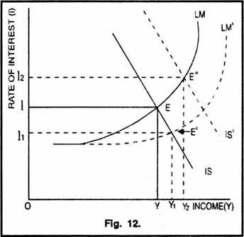
Shifts in the IS curve or the LM curve or both cause changes in the equilibrium rate of interest and the equilibrium income level accordingly. This is shown in Figure 12. The initial general equilibrium position is at point E where the IS curve and the LM curve intersect each other.
The equilibrium rate of interest is Oi and the equilibrium income level is OY. Given IS curve, if the LM curve shifts to the right (LM’), the new equilibrium point will be E’ indicating a fall in the rate of interest (from Oi to Oi1) and an increase in the income level (from OY to OY1) and vice versa. On the other hand, given the LM curve, if the IS curve shifts upward (to IS’), the new equilibrium point will be E” which indicates a rise in the rate of interest (from Oi to Oi2) and an increase in the income level (from OY to OY2) and vice versa.
To conclude, the modern theory of interest maintains that the determinants of the rate of interest along with the level of income are – (a) saving function, (b) investment function, (c) liquidity preference function, and (d) the quantity of money.
It is to be noted that Keynes’ analysis contained all these four elements, but he could not integrate them to form a determinate theory of interest. The credit goes to Hicks and Hansen for using the Keynesian tools to arrive at a complete and a determinate theory of interest.
To sum up:
The analysis of general equilibrium through IS and LM curves leads to the following conclusions:
(i) The intersection on the IS and LM curves determines the equilibrium rate of interest and the equilibrium level of income simultaneously in the product and money market.
ADVERTISEMENTS:
(ii) Any disequilibrium on the IS curve (such as points A and D on IS curve in Figure 11) is corrected through changes in the level of income. On the other hand, any disequilibrium on the LM curve (such as points C and B on LM curve in Figure 11) is corrected through changes in the rate of interest.
(iii) It follows that the IS curve indicates that changes in the rate of interest help to determine the level of income and the LM curve indicates that changes in income help to determine the rate of interest.
(iv) With a given IS curve, when LM curve shifts to the right, the rate of interest falls and the income increases; with a given LM curve, when the IS curve shifts to the right, both rate of interest and the income increase.

