
In this article we will discuss about the multiple equilibria and stability of international trade.
The offers curves of two trading countries can determine the position of general equilibrium through the intersection between them. It is possible that the equilibrium occurs not at one unique position but at several positions. Such a situation represents the multiple equilibria. Some of these equilibrium positions may not be stable. Multiple equilibria in relation to their stability is explained through Fig. 4.18.
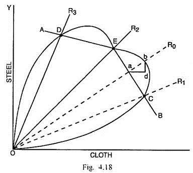
In Fig. 4.18, OA is the offer curve of country A and OB is the offer curve of country B. The intersection between them takes place at the points C, D and E indicating situations of multiple equilibria. Out of these three equilibrium positions C and D are stable while E is unstable. Any displacement from point E will give rise to such economic forces, which will either shift the equilibrium to point C or to point D. OR1, OR2 and OR3 are the international exchange ratio lines at the equilibrium positions C, E and D respectively.
ADVERTISEMENTS:
If the international exchange ratio line is OR0, the country A is willing to export ad more of cloth than what the country B is willing to have. At the same time, country A demands bd more of steel than what the country B is willing to export. Thus there is excess supply of cloth coupled with excess demand for steel. This will cause a fall in the price of cloth relative to the price of steel and the international exchange ratio line moves down towards the stable equilibrium at C.
Similarly, if there is disturbance of equilibrium from E such that the international exchange ratio line moves to the left of OR2, there will be such interaction of forces that the price of cloth will rise relative to that of steel and the two countries will move towards the stable equilibrium position at D. From the above analysis, it is amply clear that C and D are the points of stable equilibrium and E is the point of unstable equilibrium.