The New Theories of International Trade | Economics

The various traditional connoisseurs of trade theory belonging to different schools of thought such as those of Adam Smith, David Ricardo and Bertil Ohlin would at the end of the day whole-heartedly support a verdict, i.e., the verdict which asserts that each of these paradigms fabricate a logically consistent doctrine in which from certain basic premises, various theorems are deduced, concerning both positive and normative economics. Of course there are differences, major as well as minor, among the paradigms of assump­tions on which each of these trade theories is premised.

Leaving aside the assumptions specific to each model, the fundamental assumptions of the orthodox theory are:

(i) The market is perfectly competitive.

(ii) The commodities which are internationally traded are homogeneous, and identical in the various countries. This means that the homogeneous commodity A produced in country 1 is identical to the homogeneous commodity A produced in any other country, and so on for all commodities.

However in reality, these assumptions are hardly satisfied. Even a casual observation of reality shows that:

(i) Market forms different from perfect competition (such as monopolistic competition and oligopoly) are the norm rather than the exception.

(ii) Product differentiation is much more frequent than product homogeneity.

It was not as if these subtle factors had not received any attention at all from the trade theorists but the endeavors made to study these were isolated from one another and it seemed as if there was sufficient room for an analytical apparatus that would combine the fruits borne by the preceding attempts.

Such an integrated approach that embraced various individual ef­forts and synergized them into not one but rather many theories with different assumptions and consequently different results came into existence only in the 1980s.

One needs to take note of the fact that in doing so, theorists borrowed heavily from industrial economics. Thus were born the models of new theories of international trade—alias the industrial organisation approaches to international trade. The rationale behind the usage of the plural number, is, as said earlier, the emergence of not one new theory, but several, with different assumptions and results.

The common feature of these theories is that they drop the assumption of perfect competi­tion and/or of product homogeneity. In addition to this, there are two other features which are often stressed as peculiar to the new theories of trade.

These are:

(i) The explanation of intra-industry trade

(ii) The use of non-constant returns to scale.

The new trade theories can explain intra-industry trade while the orthodox theory cannot. Intra-industry trade-also known as horizontal trade or two-way trade or cross-handling-is defined as the simultaneous import and export of commodities belonging to the same industry.

This may be explained further with the help of an example. Suppose that country 1 simulta­neously exports and imports commodity A or, more precisely, similar goods belonging to the same category defined as A. Now, the kind of international trade considered by the orthodox theory can only be of the inter-industry type, i.e., exchange of products of different industries. In the conventional 2×2 setting, this means that country 1 imports one commodity, say com­modity A, and exports the other commodity B, while country 2 imports B and exports A.

In fact, according to the orthodox theory, a country cannot export and import the same good at the same time. Thus, the fact that this theory cannot explain international trade of the intra- industry type is a statement of the obvious. It is a major limitation because intra-industry trade is an important part of international trade.

This opinion, however, does not seen to be valid. Contrary to the above arguments that malign the image of the orthodox theories, it has been observed that, in several cases, the orthodox school of thought has been able to perfectly explain intra-industry trade in identical commodities.

These exceptions to the rule may be elaborated:

1. Transport Cost:

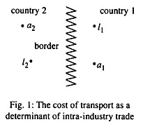
In Fig. 1 we consider two countries with a long common border and assume that they produce steel (in units situated at a₁ and a₂) which they subsequently transform into steel plate (in the units situ­ated at I₁, and l₂). It is assumed that technology, tastes and factor endowments are absolutely identical in the two coun­tries.

Ceteris paribus, if we assume that the cost of transport is directly proportional to distance, country 1 may find it cheaper to get its supply of steel from a₂, rather than a,, because a₂ is nearer to (country 1 thus imports steel from country 2) and in the same way, country 2 might find it cheaper to import steel from country 1 because as is nearer to l₂ than is a₂. Hence both countries will simultaneously import and export the same commodity (steel).

2. Periodic Trade:

This type of trade arises due to seasonal factors. Suppose that country 1 and country 2 produce the same fruit, but they are at the antipodes. Thus, in this case, we get to observe intra-industry trade on a yearly basis.

3. Varying Conditions of Demand:

It is absolutely normal for two neighbouring countries to exchange electrical power with one another to meet demand peaks in one or another country. This can be fitted into the orthodox theory, by assuming demand curves that periodically change their positions.

4. Import and Export of Goods:

Import and export of goods after storage and wholesaling (entrepot trade) or after simple manipulations (such as packaging, bottling, cleaning, sorting, etc.) which leave the goods essentially unchanged (re-export trade). Even in the case of re-export trade the manipulations are usually not sufficient to warrant the reclassification of the goods in a different SITC class, so that intra-industry trade is observed.

5. Government Intervention:

Let us assume that in a trade troika, countries 1 and 2 join a free trade area and country 2 levies higher duties against country 3 than country 1 does. It may then be advantageous for country 2, first to export the good to country 1 and so pay a lower tariff, and then re-export it to country 2 as coming from country 1, thus paying no further duties. Country 1 will then appear as an importer and exporter of the same commodity.

Now coming back to the second feature, it is claimed that the new theories of international trade can accommodate increasing returns to scale while the orthodox theory cannot. This statement is certainly true, if we consider increasing returns to scale due to external economies, which are perfectly compatible with the orthodox theory.

Only increasing returns to scale due to internal economies are incompatible with perfect competition and, hence, with the orthodox theory. Moreover, it is wrong to identify new theories as proponents of increasing returns to scale because, as shall be seen hereafter, there are many new theories that take production as occurring under constant returns to scale. Thus the quintessence of the new theories of trade as discussed above may be described as the outcome of the relaxation of the assumption of perfect competition and/or the assumption of product homogeneity.

Classification of the New Theories:

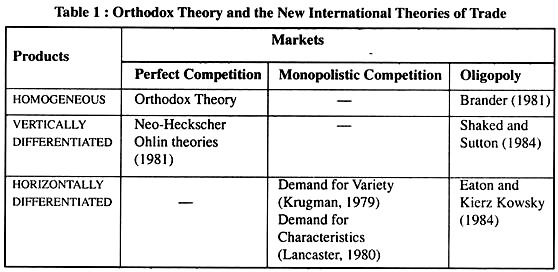
As stated earlier, we reiterate that there is not one new theory but several, with different as­sumptions and, therefore, different results. These theories may be classified on the basis of two elements: the type of good and the market form.

As far as the market forms are concerned it would suffice to say that in the “oligopoly” heading we include not only duopoly but also, as a limiting case, monopoly.

Now coming to the aspect of product differentiation it may be observed from Table 1 that product differentiation has two possible types: vertical and horizontal.

Vertical differentiation refers to products that differ only in the quality. For example, woolen suits are identical except for the quality of the wool.

Horizontal differentiation refers to products of the same quality that differ in their (real or presumed) characteristics. For example, woolen suits are often made of the same quality of wool but of different cut and colour.

In case of vertical differentiation a lot actually depends on the budget constraints of the consumers. It is common sense that all consumers would prefer higher-quality to lower-quality goods. This, of course, presupposes the existence of universally accepted criteria for evaluating quality.

Hence, in the absence of budget constraints, all consumers would demand the highest- quality good (the underlying assumption here being that the price of a commodity increases as its quality increases).

In case of horizontal differentiation, the valuation of the various characteristics differs from consumer to consumer depending on his/her perspective. It is essentially a matter of a consum­ers’ tastes and preferences. In any case, consumers do, in general, show an inclination towards variety.

It follows that the demand for different commodities, i.e., commodities having differ­ent characteristics, is related to a craving for variety and/or to different subjective evaluations of the characteristics. In fact, most commodities can differ in both quality and characteristics, but for analytical convenience we keep the two cases distinct.

We now proceed to delve into the intricacies of the post Heckscher-Ohlin theories of trade.

The Limitation Lag Hypothesis:

The imitation lag hypothesis is a brainchild of Micheal V. Posner and was formally introduced by him in 1961. In fact the intellectual supremacy of this hypothesis lies in the fact that it paved the way for another theory that was to emerge in the coming years and which is now better known as the Product Cycle Theory.

The imitation lag hypothesis drops the assumption in the Heckscher-Ohlin analysis that there is a uniformity of technologies in use across the global village. It assumes that the same technology is not always available in all countries and that there is a deferred transmission or diffusion of technology from one country to another.

Consider countries I and II. Suppose that the technocrats of country I come up with a new product, thanks to the successful endeavors of research and development teams. According to the imitation lag theory this new product will not be produced immediately by firms in country II.

Incorporating a time dimension, the imitation lag is defined as the length of time that elapses between the product’s introduction in country I and the appearance of the version produced by firms in country II.

The imitation lag includes a learning period during which the firms in country II must acquire technology and knowhow in order to produce the product. Moreover, it takes time to purchase inputs, install equipment, process the inputs, bring the finished product to market, and so on.

Moreover, there is a second adjustment lag on the demand side as well. The demand lag is the length of time between the product appearance in country I and its acceptance by consum­ers in country II as a substitute for the products they are currently using. This lag may be particularly long in case of brand loyalty products.

The central point of importance in the imitation lag hypothesis is that trade focuses on new products. How can a country become a continually successful exporter? By continually inno­vating?

An obvious advantage of this theory over the Heckscher-Ohlin counterpart is that it is more capable of handling “dynamic” comparative advantage than the latter.

The Product Cycle Theory:

The product cycle theory of trade builds on the imitation lag hypothesis in its treatment of delay in the diffusion of technology. However, the product cycle theory (PCT, hereafter) also relaxes many other assumptions of the traditional trade theory and is more complete in its treatment of trade patterns.

The PCT divides the life cycle of a new product into three stages:

(i) New product stage

(ii) Maturing product stage and

(iii) Standardised product stage

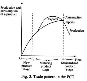
These three stages and their interaction in the world market that makes this theory opera­tional in international trade may be repre­sented diagrammatically as shown in Fig. 2.

In the first stage—the new product stage—the product is produced and con­sumed only in the home country. Firms pro­duce in the home country because that is where demand is located, and these firms wish to stay close to the market to detect con­sumer response to the product. The charac­teristics of the product and the production process are in a state of change during this stage as firms seek to familiarise themselves with the product and the market. No interna­tional trade takes place.

The second stage of the life cycle is called the maturing product stage. In this stage, some general standards for the product and its charac­teristics begin to crop up and mass production techniques are adopted. With more standardisa­tion in the production process, economies of scale stand to be realised. This is a sharp contra­diction to the Heckscher-Ohlin as well as Ricardian theories which assume the production process to be taking place under constant returns to scale.

In addition, there is a growth in foreign demand, but is associated particularly with other developed countries, since the product is catering to high income demands. The rise in foreign demand leads to a trade pattern whereby the home country exports the product to other high income countries.

Vernon suggested that in this maturing product stage, the product might now begin to flow from the foreign markets to the home country because, with capital more mobile internationally than labour, the price of capital across countries was unlikely to diverge as much as the price of labour.

With relative prices thus heavily influenced by labour costs, and with labour costs lower in foreign markets than in the home country, the foreign countries might be able to undersell the home country in this product. Relative factor endowments and factor prices, which played an important role in Heckscher-Ohlin model, have not been completely ignored in the PCT.

The final stage is the standardised product stage. By this time in the product’s life cycle, the characteristics of the product itself and of the production process are well-known; the product is familiar to consumers and the production process to producers. Vernon opined that produc­tion may shift to the developing countries. Once again, labour costs play an important role and the developed countries are busy introducing other products.

In the final diagnosis, the PCT advocates a dynamic comparative advantage because the country source of exports shifts throughout the life cycle of the product. Early on, the innovat­ing country exports the good but then it is displaced by other developed countries which, in turn, are ultimately displaced by the developing countries.

The Linder Theory:

As is evident from the nomenclature, this theory is a brainchild of the Swedish economist Staffan Burenstam Linder. The Linder theory is an exclusively demand-oriented theory as op­posed to the Heckscher-Ohlin theory which is essentially a supply side theory. The Linder theory asserts that tastes of consumers are strongly influenced by their income levels; the per capita income level of a country will yield a particular pattern of tastes.

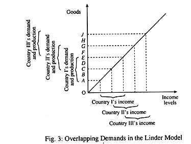
The theory may be illustrated using the following example. Suppose that country I has a per capita income level that yields demands for goods A, B, C, D, and E. These goods are arranged in ascending order of product “quality” or sophistication, with goods A and B, for example, being low-quality clothing or sandals while goods C, D, and E are further up the quality scale.

Now suppose that country II has a slightly higher per capita income. Because of its higher income, it may demand and, therefore, produce goods C, D, E, F, and G. Goods F and G may be quality products not purchased by country I’s lower-income consumers. Therefore it is evident that each country is producing goods that cater to the demands of its own citizens.

All said and done about the production patterns we may now focus the spotlight on the important question pertaining to prospects of trade between the two countries. Trade will occur in goods that have overlapping demand, meaning that consumers in both countries are demand­ing the particular items. In our example, the goods that have a scope for trade are C, D and E.

The determination of the trading pattern by observing overlapping demands has an important implication for the types of countries that will trade with each other. Suppose there is a third country involved in the above example. We assume country III’s per capita income to be even higher than that of country II.

Country Ill’s consumer demand may be for goods E, F, G, H and J. Country III will trade goods E, F and G with country II, but it will trade only good E with country I. For all three countries I, II and III in Fig. 3 portrays the income-trade relationships, recognising that there is a representative range of individual incomes around each country’s per capita income level.

In the above three-country example, the level of per capita income in country I yields a demand for goods A, B, C, D and E. Country IPs higher per capita income yields a demand for goods C, D, E, F and G and country Ill’s even higher per capita income is associated with demands for goods E, F, G, H and J. According to the Linder hypothesis, there will be an interest in trade only where income-induced product demands are similar or “overlap”.

Thus one would expect to see countries I and II trading goods C, D and E with each other and countries II and III exchanging goods E, F and G. Because their respective income levels do not generate common demands for any good except good E, countries I and III will trade with each other only in that good.

An important point concerning the Linder model is that it does not specifically assert the direction of flow of goods between the trading countries. When we stated (in the preceding example) that countries I and II would trade in goods C, D and E, we did not say which good or goods would be exported by which country. Linder opined that a good might be sent in both directions—both exported and imported by the same country.

This phenomenon was not possible in previous models of trade because it was asserted that for all practical pur­poses a country could not be said to possess a comparative advantage and a comparative disadvantage in the same good. Countries that export and import items in the same product classification are said to be engaged in intra-industry trade.

Herbert Grubel and P. J. Loyd have mentioned several reasons for the occurrence of intra-industry trade (IIT), of which few are mentioned below:

(i) Product Differentiation:

The chief reason behind the existence of a variety of products is that producers try to convert their ordinary products into brand royalty products. The objec­tive is to establish a brand equity. Consumer tastes differ in innumerable ways, more so than the varieties of products manufactured by any given country and some intra-industry trade emerges because of product differentiation.

(ii) Transport Costs:

In a large country like India, transport costs for a product may play a role in causing intra-industry trade, especially if the product has large bulk relative to its value.

(iii) Dynamic Economies of Scale:

If IIT has been established in two versions of a product, each producing firm (one in the home country, one in the foreign country) may experience “learning-by-doing” or what has been called dynamic economies of scale. This means that per unit cost reductions occur because of experience in producing a particular good.

(iv) Degree of Product Aggregation:

This explanation attributes the occurrence of IIT to the way trade data are recorded and analysed. If the category is broad, there will be greater intra-industry trade than would be the case if a narrower category is examined.

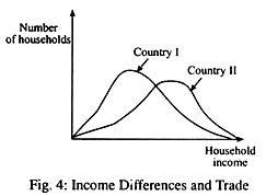
(v) Differing Income Distributions in Countries:

This explanation was offered by Herbert Grullin in 1970. He opined that even if two countries have similar per capita incomes, differing distributions of total income in the two countries can lead to intra-industry trade. Suppose there are two countries I and II with the former having a heavy concentration of households with lower incomes and the latter having a more “normal” or less skewed dis­tribution.

Producers in country I and country II, respectively, will be primarily concerned with catering to the de­mands of the consumers of their respective countries. Households in country I with a high income and those in country II with a low income would purchase the good from producers in the other country because their own home firms are not producing a variety of the good that satisfies these consumers. Hence, both countries have intra-industry trade.

The Krugman Model:

This theory of trade truly epitomizes the new generation of trade models that have come into the forefront after the demise of intellectual support for the Heckscher-Ohlin model, in letter and spirit.

The model has the following unique characteristic features that distinguishes it from the traditional models:

(i) Economies of scale

(ii) Monopolistic competition.

The Krugman model assumes labour to be the only factor of production. The internal econo­mies to the firm are incorporated in the equation for determining the amount of labour required to produce given levels of output by a firm, as shown:

L = a + bQ

where L stands for the amount of labour needed by the firm, a is a technological parameter, q is the output level of the firm, and b specifies the relation at the margin between the output level and the amount of labour needed. The equation written above has immense significance in the context of the accrual of internal economies of scale.

If a = 10, b = 2, then if the firm produces an output of 20 units, it requires 50 units of labour. Now suppose that the firm doubles its output to 40 units. The units of labour required to pro­duce 40 units of output would be 90 units. Thus, it is substantiated that the equation indicates the inherent presence of economies of scale which requires the units of labour to be less than doubled for an exact doubling of output.

It is to be noted here that the concept of advocating economies of scale shows a divergence from the traditional Ricardian model, because the latter stressed constant returns to scale. Con­sequently constant costs of production would make the relevant labour-usage equation L = bQ, i.e., the labour input has a constant relation to the amount of output.

The second main characteristic of the Krugman model is the existence of the market struc­ture of monopolistic competition. In monopolistic competition, there are many firms in the industry and easy entry and exit. Moreover, there is zero profit for each firm in the long run. However, unlike the perfect competition of traditional trade theory, the products of firms in the industry is not homogeneous. The products differ from one another, and each firm’s product possesses a certain amount of consumer brand loyalty.

According to Avinash Dixit and Joseph Stiglitz (1977) and Micheal Spence (1976) behind the demand for differentiated goods there is simply the desirability of variety as such, which is implicit in the traditional convex to the origin indifference curves.

The Krugman model heavily borrows from the preferences a la S-D-S (Spence-Dixit-Stiglitz) in his attempt to fashion this model of trade. The type of monopolistic competition Krugman has in mind to may be referred to as being essentially ‘neo- Chamberlinian’ because of its proximity to the original version of Chamberlin.

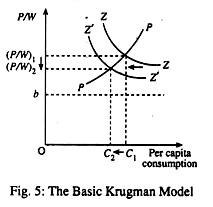
The Krugman model is most easily portrayed through Krugman’s basic graph.

The horizontal and vertical axes show the consumption of a typical good by any representative consumer in the economy, that is, per capita consumption, c and the ratio between the price of the good and the wage rate, respectively.

The ZZ curve indicates the phenomenon in monopolistic competition that economic profit for a firm is zero in the long run.

The upward sloping PP curve indicates that as per capita consumption (C) of the good rises, the price of the good will rise. The reason is that demand is assumed to become less elastic as consumption increases, and thus the profit-maximising price P = MC [_ep /(e_p + 1)]. The downward sloping ZZ curve reflects the fact that profit in the long run is zero.

With the opening up of trade the market size is enlarged because each representative firm now has more potential buyers. When the market size is enlarged economies of scale come into play and production costs are reduced for all goods.

If the firm being considered is in country I, the opening of the country to trade with country II means that consumers in both countries are now consuming this product (as well as other products)—country. II’s consumers now add country I products to their consumption bundle, just as country I’s consumers add country II’s products to their consumption bundle.

If the firm’s total output is momentarily held constant, there is thus, with the larger consuming population but with the spreading out of consumption to other, newly available products, less per capita consumption of this firm’s product at each P/ W than was previously the case. This is equivalent to a leftward shift of the ZZ curve, repre­sented by the ZZ curve in Fig. 5.

Given the shift of ZZ to Z’Z’, there is thus disequilibrium at the old equilibrium point E, and movement from E to E’ leads to a fall in the (PAV) ratio from (P/W), to (P/W)₂ as shown in the Fig. 5. Although per capita consumption also falls from C₁to C₂, the magnitude of decrease in consumption is lesser than the quantum of increase in size of the consuming population, imply­ing that total consumption of the firm’s product has increased; with this increased output by the firm the scale economies have come into play and have reduced unit costs.

As is visible from both the theoretical and the diagrammatic versions of reasoning, the PAV in this country has undergone a reduction. This obviously means that the W/P ratio has in­creased. The wage to price ratio is nothing but the real income of consumers. So there is a manmade improvement on the front of the real income of workers as well.

Moreover, unlike the H-O model where the scarce factor of production is set to lose from trade, the gain that persists in the Krugman model—both from a higher real wage due to the economies of scale and from the increased variety of goods due to product differentiation- more than compensates the loss. Hence the bottom line is that the “gainer loser” income distri­bution aspects do not come into play of trade consists of an exchange of differentiated products produced under conditions of economies of scale.

The Gravity Model:

The gravity model owes its birth to the efforts of several neo-Heckseher-Ohlin trade theorists such as Tinbergen (1962), Poyhonen (1963), Linnemann (1966), Deardorff (1984), Teamercud Levinsohn (1995) and Helpman (1999). It differs from most other theories is that it is trying to explain the volume of trade and does not focus on the composition of that trade.

The model itself uses an equation framework to predict the volume of trade on a bilateral basis between any two countries. The similarity of the structural form equation of the model to the law of gravity has led to the nomenclature of the “gravity model”. It is concerned with selecting economic variables that will produce a “good fit”, that D, that will explain at least in a statistical sense a substantial portion of the size of trade that occurs.

The variables that are nearly always used in the equation as causes of flow of experts from a country I to country II are:

(i) A national income variable for country II (GNP or GDP), which is expected to be directly proportional to the volume of exports from I to II because higher income in II would cause II’s consumers to buy more of all goods, including goods from country I.

(ii) A national income variable for country I (GNP or GDP), reflecting that greater income in I means a greater capacity to produce and, hence, to supply, exports from I to II.

(iii) Some measure of distance between country I and country II as a proxy for transporta­tion charges with the assumption that distance is inversely proportional to the volume of ex­ports from country I to country II.

Sometimes, other variables such as population size in the exporting and/or importing coun­try, the economies of scale due to a larger market size or a variable showing an economic integration arrangement such as an FTA (free trade area) are also introduced.

Empirical tests using the gravity model have till date enjoyed stupendous success. The gravity equation worked best for similar countries that had considerable intra-industry trade with each other, than it did for countries with different factor endowments and a predominance of inter ­industry trade rather than intra-industry trade.

Conclusion:

The analysis of the five points of the Heckscher-Ohlin model conclusively proves that the criticisms surrounding them is not without reason because traditional trade theories have ne­glected some aspects such as economies of scale, product differentiation, market imperfections and intra-industry trade that leaves much more to be accomplished in these directions.

Basically we have viewed five new theories that embrace the concepts of lags in diffusion of technology, demand considerations, economies of scale and dynamic comparative advantage.

These theories have some interesting implications for the developing countries. The imita­tion lag hypothesis and the product cycle theory do not lead to particularly optimistic result about the future export performance of developing countries because they suggest that de­veloping countries may remain confined to exporting older products rather than new high- technology goods.

But there are some positives to be drawn as well. Developing countries like India and the rest of the countries from the Asian subcontinent can take a leaf out of the book of the five “Asian Tigers” and shift their focus from exporting primary products to exporting manufactured products.

Theories of Linder and Krugman carry the message that trade will increasingly take place between countries having similar income levels. Finally, these models indicate the difficulty of predicting future trade patterns but suggest potentially large gains from trade.