Expenditure Function of Investment (With Diagram)

In this article we will discuss about the Expenditure Function of Investment.

Recall that the only two kinds of output produced-i our hypothetical economy are consumption goods and capital (investment) goods. Thus total de­sired spending in this two-Sector economy must be the sum-total of desired consumption expenditure and desired investment expenditure. Thus: E = C + I. where E is total desired spending.

It is now instructive to enquire how changes in na­tional income affect the total desired expenditure of households and business firms. In our simple model investment has been assumed to be autonomous and hence independent of national income. Thus aggre­gate desired expenditure varies with national exactly as does desired consumption spending.

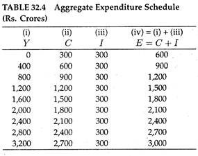
Table 32.4 illustrates how we arrive at the aggre­gate expenditure function. Here we use the same set of data on consumption and income as presented in Table 32.1.

We also make the added assumption here that investment is constant at Rs. 300 crores. Column (1) along with column (4) shows how desired aggre­gate expenditure varies as national income changes. These two columns define the aggregate expenditure function, which shows how much business firms and households like to spend on purchasing final goods at each level of income.

This function shows how much of the economy’s output is demanded by these two groups and is also often called an aggregate demand function. Since our focus is on the total amount house­holds and firms wish to spend on the economy’s out­put, we prefer to use a term ‘aggregate expenditure function’.

A. Graphical Representation of the Expenditure Function:

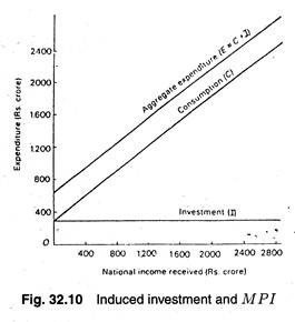
The consumption and investment functions given in Table 32.4 are illustrated in Fig. 32.10. On the basis of these two functions we derive the aggre­gate expenditure function. In fact, the aggregate ex­penditure (C + I) function is the vertical summation of the individual expenditure function the consump­tion function (C) and the investment function (I).

It is quite obvious that the vertical summation of the C + I curves is the geometrical equivalent of adding columns (ii) and (iii) in Table 32.4 and Fig. 32.10 show different C + I values associated with each level of income.

Shifts in the Aggregate Expenditure (C + l) Func­tion:

We have noted that the aggregate expenditure function is the sum of the consumption and investment functions. Therefore anything that shifts either of the functions will shift the aggregate expenditure function. We may now consider shifts of C and I functions one by one.

Consumption:

A change in income leads to a movement along the same consumption function. While developing a stable income-consumption re­lation we held all other factors constant. However, in practice these other variables keep on changing. And a change of any other variable affecting consumption spending will shift the consumption function upward or downward.

The consumption function may shift upward due to the following:

1. A reduction in the thriftiness of the people.

2. A fall in the rate of interest which reduces the reward for saving.

3. A fall in the rate of interest which induces people to buy now before prices rises.

4. An increase in the stock of wealth so as to make people feel that it is less urgent and important to save in order to add to their stock of wealth.

In short, anything that increases (decreases) the desire to spend on consumption good and hence re­duces (increases) the desire to save will cause an up­ward (downward) shift of the consumption function and a corresponding upward (downward) shift of the aggregate expenditure function.

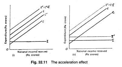
The effect of an upward shift in C and C + I functions is shown in Fig. 32.11 (i). The initial con­sumption function is labelled C. The increased desire to consume shifts the function upward to C’. (The investment function here remains unchanged).

This indicates a high level of desired consumption spend­ing at each level of national income. This also lead to a shift of the aggregate expenditure function upward by the same amount, from E to E’.

The converse is also true. The same figure may also be used to show a downward shift of the con­sumption and aggregate expenditure function.

All the four factors listed above will influence the consumption and saving decision of each house­hold and hence influence aggregate consumption be­haviour, too. However, another factor will affect ag­gregate consumption behaviour, viz., a redistribution of income among households. Income redistributions can shift the aggregate consumption functions of the individual households.

In general the poor people have a stronger pro­pensity to consume that the rich people. Thus if in­come is redistributed from the rich to the poor ag­gregate consumption spending will rise. This is why Keynes himself was in favour of such redistribution during depression.

In short, “redistribution of national income will shift the aggregate consumption function upwards if those gaining the income have higher MPCs than those losing it, and downward if those gaining the income have lower MPCs than those losing it.”

Investment:

In Keynes’ model investment is an autonomous expenditure flow. This is why the in­vestment schedule I is horizontal, parallel to the hor­izontal axis. Thus a fixed level of investment takes place at each level of national income.

However, a change in any of the forces that influ­ence desired investment spending will change the vol­ume of investment.

The investment function I may shift upward due to the following:

1. A fall in the rate of interest

2. An increase in MEC

3. Improved sales prospects (expectations)

4. Expectations of decreased costs in the future and

5. A rise in profits which can be used to finance investment.

Opposite changes will cause a fall in desired in­vestment spending and the investment function I will shift downward in this case.

In Fig. 32.11 (ii) there is an upward shift of the investment function from I to I’. The consumption function remains unchanged. Consequently, the ag­gregate expenditure functions shifts by the same amount—from E to E’. In the converse case the in­vestment functions would have shifted downward. This could also be shown in the diagram.