How to Obtain Equilibrium of Economy using IS and LM Curve?

The following article will help you to know how to Obtain Equilibrium of Economy using IS and LM Curve.

Equilibrium in the economy occurs when both the money market and the product market are simultaneously in equilibrium.

These two large markets interact, and the adjustments that occur in either of the markets will induce adjustments in the other market.

For example, if product market conditions change and this alters the level of real output, the demand for real money balances will change inducing adjustments in the market real rate of interest.

Similarly, if conditions in the money market change, causing an adjustment in the market real rate of interest, the level of investment demand will change. This change in the level of aggregate demand will then induce a change in the level of real output in the product market. The interaction between these two markets can be analysed with the use of the IS and LM curves.

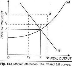
The IS curve represents the relationship between the level of real output and the real interest rate, which generates equilibrium in the money market. These curves, for given levels of government expenditure, taxation, net exports, prices, and anticipated rate of price change are shown in Figure 14.4. Any changes in the conditions that are assumed given for these two curves would be shown as shifts in either the IS or the LM curve.

Suppose that the economy was initially at a real interest rate of r₂ and a level of real output of Y₂. This is shown by position a in Figure 14.4. At a, both the product market and the money market are out of equilibrium. For the real interest rate of r₂ there is not sufficient aggregate demand for real output to sustain the real income level of Y₂.

Equilibrium in the product market for a real interest rate of r₂ would occur at the level of real output Y₁. At point a there is a deficiency of aggregate demand. The unintended inventory accumulation will induce producers to cut back on their production. As a result, real income and employment will decline.

Similarly, at the real income level of Y₂, the real interest rate of r₂ is too high for equilibrium in the money market. At point a there is an excess supply of real money balances. Credit conditions will change as individuals attempt to remove these excess holdings of real money balances by acquiring additional bonds, and the market real rate of interest will decline.

Both markets will continue to adjust until simultaneous equilibrium is reached. This equilibrium position for both the product and money markets is given by the intersection E of the IS and the LM curves at the real income level Y with the real interest rate r.

Points off the IS Curve:

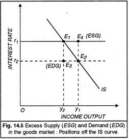
Let us now try to understand as to what happens when the economy is in disequilibrium, say on a point off the IS curve. In Figure 14.5, we have the points E₃ and E₄ which are not on the IS curve. At these points, the goods market is not in equilibrium. So, what is the position of the goods market? Take the point E₃. This point is to the left of the IS curve. The economy’s output implied in this combination is shown by the level and the rate of interest r₂. At the r₂ level of the rate of interest, the real demand for output is that shown by Y₂ which means an excess demand for goods (EDG) at the point E₃.

The economy will tend to go to the position E₂. Likewise, at the point E₄, the level of output implied is Y₂ with the real rate of interest at the level. Since this point is off the IS curve, it shows disequilibrium in the goods market. At the rate of interest shown by r₁, people are prepared to purchase only Y₁ level of output while the actual output associated with E₄ is Y₂. So, there is excess supply of goods at the point E₄. The economy will tend to go to the position E₁ so as to restore the goods market equilibrium.

Points off the LM Curve:

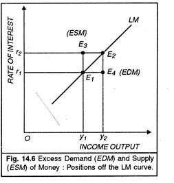
We know that the money (assets) market is in equilibrium when the output and rate of interest are such as to equate the demand for money with the supply of money. In Fig. 14.6, the points E₁ and E₂ show the equilibrium positions of the money market with appropriate combinations of output and the real rate of interest. Now, what happens if the economy is on the point E₃ or at the point E₄? The point E₃ is to the left of the LM curve.

At this high rate of interest r₁ associated with E₃, there is excess amount of money supply (ESM). This is clear from the fact that the money supply implied in E₃ can support the output Y₂ while the rate of interest associated with E₃can support the output Y₁ only. As a result the rate of interest will have to fall to induce higher investment and demand for money to eliminate the excess supply of money.

Likewise, we can argue the position of the point E₄ which is to the right of the LM curve. This point combines r₁ rate of interest with Y₂ level of income. Now this combination is not maintainable because it shows excess demand for money on the part of households and firms.

The money supply available is that shown by E₁ while the demand for money as originating from the output Y₂ is that shown by E₄. Clearly, there is excess demand for money which will have to be adjusted by changes in the rate of interest and output at the same time.