Intersection of the IS Curve with the LM Curve (With Diagram)

Intersection of the IS Curve with the LM Curve!

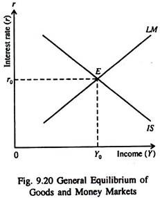
Any point on the downward sloping IS curve shows commodity market equilibrium. Similarly, any point on the upward sloping LM curve shows money market equilibrium. And money market equilibrium implies equilibrium of the bond market. The two curves meet at point E, which shows the general equilibrium of commodity mar­ket and money market. It shows how Y and r are determined simultaneously.

In Fig. 9.20, r₀ and Y₀ are the equilibrium values of rate of interest and income that ensure equilibrium of virtually three markets at the same time, viz., the commodity market, the money market and the bond market.

The nature of this general equilibrium can be un­derstood better by considering whether the IS-LM model is stable or not. In order to test the stability aspect of the model we have to examine whether any deviation from the equilibrium point E tends to create forces that bring the system back to equilibrium, i.e., whether any deviation from point E is followed by an immediate return to it.

Examples:

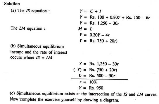
2. Consider a two-sector model where C = Rs. 100 + 0.80yY and I = Rs. 150 – 6r, M = Rs. 150 and L = 0.20Y – 4r.

(a) Find an equation for equilibrium in the goods market (IS) and for the money market (LM).

(b) Find the income level and rate of interest at which there is simultaneous equilibrium in the money and commodity markets.

(c) Plot the IS and LM equations in a diagram and find the equilibrium income and the rate of interest.

3. The equation for equilibrium in the goods market is Y = Rs. 1,250 – 30r and in the money market Y = Rs. 750 + 20r when

Find out equilibrium Y and r as also the effect of an increase in money supply of Rs. 10.

Solution:

Simultaneous equilibrium in the money and goods markets exists at a 10% rate of interest and Rs. 950 income level. A Rs. 10-increase in the money supply, holding the income level constant at Rs. 950, lowers the rate of interest from 10 to 7.50%:

Rs. 160 = 0.20 (Rs. 950) – 4r

or, 4r = Rs. 30 or, r = 7.50%

However, a lower interest rate increases investment spending and, through a multiplier effect, equilibrium income. Simultaneous equilibrium in the money and the goods markets is restored when the income level increases from Rs. 950 to Rs. 980 and the rate of interest from 7.5 to 9%.

Y = Rs. 1,250 – 30r (IS equation)

(Y = Rs. 760 + 20r) (LM equation when money supply is Rs. 160)

0 = Rs. 490 – 50r

r = 9.8%

Y = Rs. 956

Thus, the Rs. 10-increase in the money supply causes a liquidity effect which reduces the rate of interest from 10 to 7.5%; the resulting income effect then increases the rate of interest from 7.50 to 9.8%.

3. Consider a two-sector economy where the IS equation is Y = Rs. 1,250 – 30r.

(a) Given a Rs. 150 money supply, find equilibrium when the LM equation is (1) Y = Rs. 750 + 20r (where L = 0.20 K – 4r) and (2) Y = Rs. 600 + 35r (where L = 0.25 Y – 8.75r).

(b) What happens to equilibrium income and the rate of interest for situations (1) and (2) when the money supply increases by Rs. 20?

Solution:

(a) Equilibrium income is Rs. 950, and the rate of interest is 10% for situations (1) and (2).

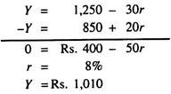
(b) For situation (1), the Rs. 20 money supply increase shifts the LM curve rightward by Rs. 100, that is, ΔM̅ (I / k) = Rs. 20/(0.20). Equilibrium income increases from Rs. 950 to Rs. 1,010; the rate of interest falls from 10% to 8%.

For situation (2), the Rs. 20 money supply increase shifts LM rightward by Rs. 80, for Δ M̅(1/k) = 20/0.25. Equilibrium income increases from Rs. 950 to Rs. 986.90; the rate of, interest declines from 10 to 8.76%.

i. Stability of the Model:

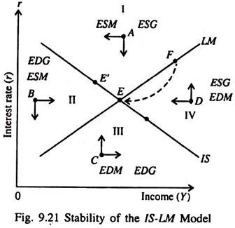
In Fig. 9.21 we show four points off the IS and LM curves (A, B, C and D). At this stage it may be noted that to the right of the IS curve there is excess supply of goods (ESG) and to the left of the IS curve there is ESG. Since it is a fixed-price model, excess demand for goods (EDG) will lead to output expansion and ESG will lead to output contraction.

To the left of the LM curve, there is excess supply of money (ESM) which will cause r to fall and to the right of the LM curve there is excess demand for money (EDM) which will cause r to rise. We see that if there is any deviation from point E, and the economy moves to, say, point F, it will come back to point E, in a cyclical manner though, as is indicated by the arrows in quadrant IV.

The stability property may be explained further:

First, let us consider points A and B above the LM curves. There is ESM because, the corresponding r is too high for money market equilibrium. As a result r has to fall and there is a tendency for the macro-economy to move toward the LM curve. Conversely, at points below the LM curve, such as C and D, there is EDM which will cause r to rise, as is pointed out by the two upward pointing ar­rows.

Now we consider two points B and D, lying above the IS curve, where there is ESG, i.e., output exceeding aggregate demand or saving plus taxes exceeding investment plus government expenditure (S + T > I + G). As a result Y will fall.

At point A there is ESM which will cause r to fall, as is shown by the downward pointing arrow. The converse is also true. At points such as B and C, which also lie below and to the left of the IS curve, there is EDG.

This means that actual output is less than the level that clears the goods market. So output (income) has to rise to meet the excess demand as is indicated by the rightward pointing arrows. At interest rate indicated by either B or C, the corresponding output level that will equate I + G with S + T, as given by the point along the IS curve, is below the actual output level. Since there is ESG, Y will rise.

At point B there is EDG which will cause Y to rise. Moreover the ESM will cause r to fall. At point C there is EDG which will cause r to rise, as is pointed out by the upward pointing arrow.

However, a point like F on the LM curve shows money-cum-bond market equilibrium, but since it is not on the IS curve, it shows commodity market disequilibrium. This point may be compared with point A or D which is off both the curves and shows disequilibrium in both the markets. Since point F is off the IS curve and lies above and to the right of the IS curve, there is ESG. This will cause output to fall, aggregate price level remaining the same.

Similarly, any point on the IS curve other than E such as E’ shows commodity (goods) market equilibrium, but money market disequilibrium since it is off the LM curve. Since this point lies above and to the left of the LM curve there is ESM — which will cause the rate of interest to fall. Only at point E are both the markets in equilibrium at the same time.

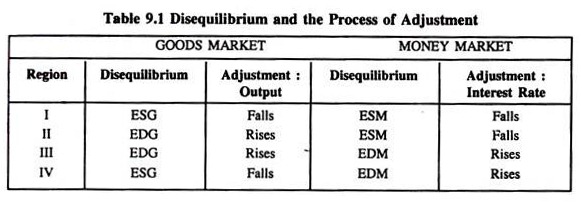
The equilibrium condition of the IS-LM model is satisfied only at this point where there is neither excess demand nor excess supply in any one of the two markets – the goods market and the money market. So there is neither upward nor downward pressure on the level of income or on the rate of interest. The nature of disequilibrium and the types of adjustment in the two markets are summarised in Table 9.1.

ii. Stability of the IS-LM Model in Light of Different Speeds of Adjustments of Output and Interest:

We know that the IS-LM model is inherently stable. Any disequilibrium — either in the money market or in the commodity market or in both the markets — will lead to restoration or equilibrium, perhaps in a cyclical manner. Both Y and r adjust to restore equilibrium in both the markets.

However, at times it is both useful and instructive to restrict the dynamics of the IS- LM model by the reasonable assumption that the money market adjusts very fast and the commodity market (i.e., the market for goods and services) adjusts slowly.

Since the money market can adjust merely through the buying and selling of bonds, it is fair enough to assume that the interest rate adjusts rapidly and the money market is always in equilibrium. This simply means that the economy is always on the LM curve: any departure from the equilibrium in the money market is immedi­ately eliminated by an appropriate change in the interest rate.

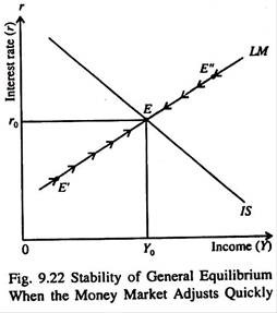
In disequilibrium, the eco­nomy, therefore, moves along the LM curve as shown in Fig. 9.22. The goods market adjusts relatively slowly because firms require some time to adjust their output levels.

For points below the IS curve, the economy moves along the LM curve with rising income and interest rates and for points above the IS curve, the economy moves down along the LM curve with falling output and interest rates until both the markets reach point E. The adjustment process is stable in the sense that the economy moves to the equilibrium point E as usual.

Suppose the economy is to the left of the IS curve say at point E’. There is excess demand in the commodity market. This will cause Y to rise. As a result there will be an excess demand for money. As Y increases L(Y, r) increases above M (money supply). This implies that L > M.

Then r will rise immediately so that L(Y, r) falls to keep the money market in
equilibrium. Since the money market clears instantaneously, r will increase in response to excess demand for money so that M is equated L(Y, r). The economy will move along the LM curve from E’ to E, raising both Y and r.

The logic of the adjustment process is simple. To the right of the IS curve, there is an excess supply of goods and firms are, therefore, having undesired inventories. This will force them to cut production. Consequently the economy moves down the LM curve. As the economy moves toward the equilibrium level of income, with a falling interest rate, desired investment spending rises as the interest rate falls.