IS-LM Curve (With Diagram): An Overview

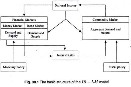
The below mentioned article provides an overview on IS-LM Curve.

The Goods Market and the IS Curve:

The goods market equilibrium schedule is the IS curve (schedule). It shows combinations of interest rates and levels of output such that planned (desired) spending (expenditure) equals income.

The goods- market equilibrium schedule is a simple extension of income determination with a 45° line diagram. Now investment is no longer fully exogenous but is also determined by the rate of interest (which is a policy variable).

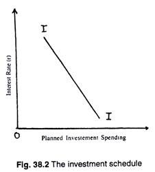
Fig. 38.2 shows a typical investment (demand) schedule. It shows the planned level of investment (spending) at each rate of interest. Since higher rates of interest reduce the profitability of additions to the capital stock, they imply lower planned rates of in­vestment spending. (Changes in autonomous invest­ment shift the investment schedule).

The investment function is expressed as: I = I̅ — cr, c > 0, where r is the rate of interest and measures the interest response of investment. I̅ denotes autonomous in­vestment, that is, investment spending which is inde­pendent of both income and the rate of interest.

The investment function above states that the lower the interest rate, the higher is planned investment, with the coefficient c measuring the responsiveness of in­vestment spending to the interest rate.

Fig. 38.3 shows how the IS curve is derived. At an interest rate, r₁ equilibrium in the goods market is at point E in the upper part of the figure, with an income level of Y₁. In the lower part of this diagram we show point E’. Now a fall in the interest rate to r₂ raises aggregate demand, increasing the level of spending at each income level.

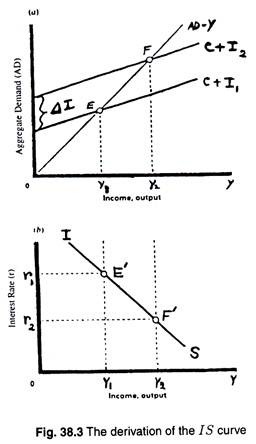
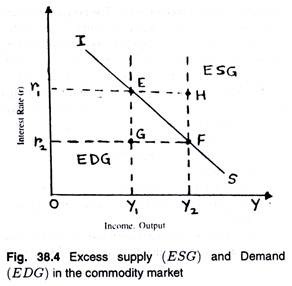
The new equilibrium income is Y₂. In the lower part, point F shows the new equilibrium in the goods market corresponding to an interest rate r₂. The IS curve is a locus of points showing alternative combinations of interest rates and income (output) at which the commodity market clears. That is why the IS curve is called the commodity market equilibrium schedule.

We can gain further insight into the IS curve by raising and answering the following questions:

1. What determines the slope of the IS curve?

2. What determines the position of the IS curve, given its slope, and what causes the curve to shift?

3. What happens when the interest rate and income are at levels such that we are off the IS curve?

Properties of the IS Curve:

1. The Slope of the IS Curve:

The IS curve is negatively sloped because a high­er level of the interest rate reduces investment spend­ing, thereby reducing aggregate demand and thus the equilibrium level of income. The steepness of the curve depends on the interest elasticity of investment (i.e., how sensitive investment spending is to changes in the interest rate) as also on the (investment) multi­plier.

2. The Position of the IS Curve:

The position of the IS curve depends on the level of autonomous spending. If autonomous spending increases, the IS curve will shift to the right (with or without a change in slope, depending on interest elasticity of investment).

3. The Positions off the IS Curve:

Fig. 38.4 is just a reproduction of Fig. 38.3(b), along with two additional points—the disequilibrium points G and H. At point G national income is the same as at E, but the rate of interest is lower (r₂).

Consequently the demand for investment is higher than that at E, and the demand for commodities is higher than that of E. This simply means that the de­mand for goods must exceed the level of output, and so there is an excess demand for goods (EDG). Likewise, at point H, the rate of interest is higher than at F. and there is excess supply of goods (ESG).

Thus Fig. 38.4 clearly shows that points above and to the right of the IS curve like H, are points of excess supply of goods (ESG). By contrast points below and to the left of the IS curve are points of excess demand for goods (EDG). At a point like G, for instance, the interest rate is too low and aggregate demand is too high relative to output.

Major Points About IS Curve:

The main points about the IS curve are the fol­lowing:

1. The IS curve is the schedule of combinations of the interest rate and the level of income such that the goods market is in equilibrium.

2. The IS is negatively sloped because an increase in the interest rate reduces planned (desired) in­vestment spending and therefore reduces aggre­gate demand, thereby lowering the equilibrium level of income.

3. The smaller the multiplier and the less sensitive investment spending is to changes in the interest rate, the steeper the IS curve.

4. The IS curve is shifted by changes in autono­mous spending. An increase in autonomous spending, such as investment spending or gov­ernment expenditure, shifts the IS curve to the right.

5. At points to the right of the IS curve, there is excess supply in the goods market: at points to the left of the curve, there is excess demand for goods.

Money Market Equilibrium and the LM Curve:

The financial market refers to the market in which money, bonds, stocks, and other forms of income- earning assets are traded. Here we restrict ourselves to the money market.

To study equilibrium in the money market, we have to refer to both sides of the market—the supply side and the demand side. The supply (or nominal quantity) of money (M) is deter­mined by the Central Bank. So we assume it to be given at the level M.

Fig. 38.5 shows the demand for money as a func­tion of the interest rate and real income. The money demand function is expressed as: L = kPY — hr, k. h > 0. The parameters k and h reflect the sensitivity of the demand for money to the level of in­come (Y) and the interest rate (r), respectively.

[Here kPY is transaction-cum-precautionary demand for money and hr is speculative demand.] The demand for money (liquidity preference) is drawn as a func­tion of the rate of interest (r).

The higher the rate of interest, the lower the quantity of money demanded, at a fixed level of income. An increase in income raises the demand for money. This is shown by a rightward shift of the money demand schedule.

Fig. 38.6 shows how the LM curve is derived. The right hand diagram [part (b)] shows the money market. The supply of money is the vertical line M, since it is fixed by the Central Bank. The two demand for money curves L₁and L₂ correspond to two dif­ferent income levels. When the income level is Y₁, the demand curve for money is L₁ and the equilibrium rate of interest is n.

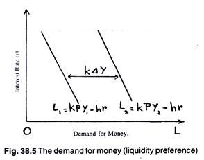
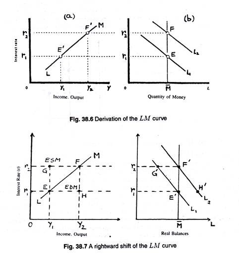
This gives point E’ on the LM schedule in part (a). At a higher income level (Y₂); the equilibrium rate of interest is r₂, yielding point F’ on the LM curve.

The LM curve is a locus of points showing alternative combinations of the rate of in­terest and the level of income that brings about equilibrium in the money market. In other words, the LM schedule (curve), or the money market equilibrium schedule, shows all combinations of interest rates and levels of income such that the demand for money is equal to its supply.

Properties of the LM Curve:

We may now briefly discuss the properties of the LM schedule.

These are the following:

1. The Slope of the LM Curve:

The LM schedule is positively sloped. This means that an increase in the interest rate reduces the demand for money. To maintain the demand for money equal to the fixed supply, the level of income has to rise. Accordingly, money market equilibrium implies that an increase in the interest rate is accom­panied by an increase in the level of income.

The greater the responsiveness of the demand for money to income, as measured by k, and the lower the responsiveness of the demand for money to the interest rate, as measured by h. the steeper the LM curve will be.

In fact, a given change in income, ∆Y, has a larger effect on the interest rate, r, the larger is k, and the smaller is h, If the demand for money is fairly inelastic, so that h is close to zero, the LM curve is nearly vertical.

If the demand for money is fairly elastic (i.e., very sensitive to the interest rate), so that h has a high value, then the LM curve is almost horizontal. In that case, a small change in the interest rate must be accompanied by a large change in the level of income in order to maintain money market equilibrium.

2. The Position of the LM Curve:

The money supply is held constant along the LM curve. It follows then that a change in the money sup­ply shifts the LM curve. This point is illustrated in Fig. 38.7. An increase in the quantity of money in circulation shifts the supply curve of money to the right in part (b)—from M₁ to M₂.

To restore money market equilibrium at the initial level of income Y₁, the equilibrium rate of interest in the money market has to fall to r₂. In part (a) we show point F’ as one point on the new LM schedule, corresponding to the higher money stock.

Thus an increase in the money stock shifts the LM curve to the right. At each level of income the equilibrium interest rate has to be lower to induce people to hold the larger quantity of money. Alternatively, at each level of interest rate the level of income has to be higher so as to raise the (trans­actions) demand for money and thereby absorb the extra money supplied.

3. Positions off the LM Curve:

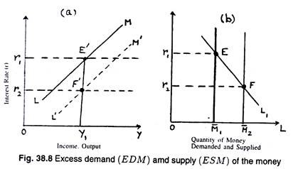
Fig. 38.8 shows points off the LM curve. Points above and to the left of the curve correspond to an excess supply of money; points below and to the right, to an excess demand for money.

Starting from point E in part (a), an increase in income takes us to point H. At H’ in part (b) there is an excess demand for money—and thus at H in part (a), there is an excess demand for money. By similar argument, we can start at F’ and move to G’ at which the level of income is lower. This creates an excess supply of money.

The following are the major points about the LM curve:

1. The LM curve is the schedule of combinations of interest rates and levels of income such that the money market is in equilibrium.

2. The LM curve is positively sloped. Given the fixed money supply, an increase in the level of income, which increases the quantity of money demanded, has to be accompanied by an increase in the interest rate. This reduces the quantity of money demanded and thereby maintains money market equilibrium.

3. An increase in money supply shifts the LAI curve to the right.

4. At all points to the right of the LAI curve, there is an excess demand for money, and at points to its left, there is an excess supply of money.

Macro-Economic General Equilibrium:

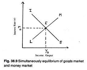
We may now discuss the joint equilibrium of both markets in order to see how output and interest rates are determined simultaneously. For simultaneous equilibrium, interest rates and income levels have to be such that both the goods market and the money market are in equilibrium.

Fig. 38.9 shows that the interest rate and the level of output are determined by the interaction of the money (LM) and commodity (IS) markets. Both markets clear at point E. Interest rates and income levels are such that the public holds the existing quantity of money, and planned spending (or desired expenditure) equals output (GNP).

Changes in the Equilibrium Levels of Income and the Interest Rate:

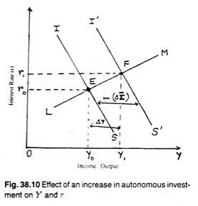
The equilibrium levels of income and interest rate change when either the IS curve or the LM curve shifts to a new position (either to the right or to the left). Fig. 38.10, for example, shows the effects of an increase in autonomous spending (such as autono­mous investment) on the equilibrium levels of income and the interest rate. An increase in autonomous spending shifts the IS schedule to the right.

As a result national income increases, and the equilibrium level of national income rises. But the increase in in­come (∆Y) is less than that given by the Keynesian investment multiplier [m (∆I] because interest rates increase and choke off investment demand.

The rea­son is easy to find out. The increase in autonomous spending no doubt tends to increase the level of in­come. But an increase in income increases the demand for money.

With a fixed supply of money, the interest rate has to rise to ensure that the demand for money stays equal to the fixed supply. When the interest rate rises, investment spending is reduced because investment is negatively related to the rate of interest (dl/dr < 0).

Adjustment toward Equilibrium:

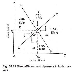
Suppose our hypothetical economy were initially at a point like E in Fig. 38.10 and that one of the curves then shifted, so that the new equilibrium was at a point like F. How would that new equilibrium actually be reached? The adjustment would involve changes in both the interest rate and the level of in­come.

Here we make two assumptions:

(1) Since prices are assumed to remain fixed, when demand increases output increases, and output falls when de­mand falls. This follows from the Keynesian theory of income determination.

(2) The interest rate rises when there is an excess demand for money and falls when there is an excess supply of money. (This follows from the Keynesian liquidity preference theory). Fig. 38.11 shows how they move over time. Four regions are shown in this diagram and they are characterized in Table 38.1.

We know (from Fig. 38.8) that there is an excess supply of money above the LM curve, and hence we show ESM in regions I and II in Table 38.1. Similarly we know (from Fig. 38.4) that there is excess demand for goods below the IS curve. Hence, we show EDG for regions II and III in Table 38.1. The remaining entries of Table 38.1 can be explained in a similar way.

The directions of adjustments are represented by arrows. Thus, for example, in region IV we have an excess demand for money, which causes interest rates to rise as other assets (including stocks and bonds) are sold off for money and their prices decline.

The rising interest rates are represented by the upward-pointing arrow. There is also an excess supply of goods in re­gion IV and, accordingly, involuntary inventory accu­mulation, to which producing units (firms) respond by reducing output. Declining output is indicated by the leftward-pointing arrow.

The adjustments shown by the arrows will lead ultimately, perhaps in a cycli­cal manner, to the equilibrium point E. For example, starting from F, we show the economy moving to E, with income and interest rate increasing along the ad­justment path indicated.

In short, income and interest rates adjust to the disequilibrium in goods markets and assets (money) markets. Specifically, interest rates fall when there is an excess supply of money and rise when there is an excess demand. Income rises when aggregate demand for goods exceeds output, and falls when aggregate demand is less than output. The system ultimately moves to the equilibrium point at E.

Use of the Model:

The IS — LM model continues to be used (since its introduction in 1939 by J. R. Hicks) for macro- economic studies. The main reason is that it provides a simple and appropriate framework for analysing the effects of monetary and fiscal policy changes on the demand for output and interest rates.

Problem 1:

Given:

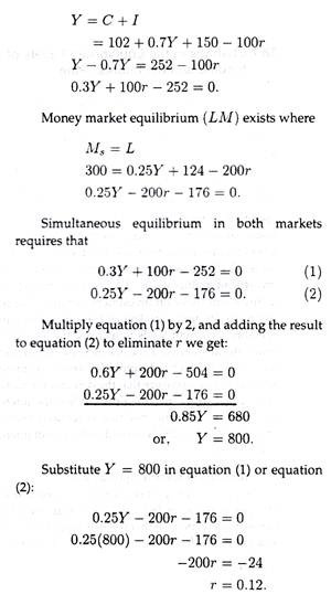
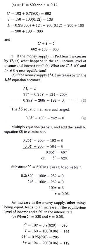
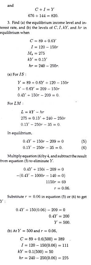
C = 102 + 0.7Y. I = 150 – 100r.M_s = 300, L = 0.25F + 124 – 200r of which kPY = 0.5y and hr = 124 – 200r. Find (a) the equilibrium level of income and the equilibrium rate of interest, and (b) the level of C, I, and L when the economy is in equilibrium.

Solution, (a) Commodity market equilibrium (IS) exists where

 

 

 

 

 

 

 

 

 

 

 

 

 

 

 

 

 

 

 

 

  

 

 

 

 

 

 

 

 

 

 

 

 

 

 

 

 

 

 

 

 

 

 

 

 

 

 

 

 

 

 

 

 

 

 

 

 

 

 

 

 

 

 

 

 

 

 

 

 

 

 

 

 

 

 

 

 

 

 

 

 

 

 

 

 

 

 

 

 

 

 

 

 

 

 

 

 

 

 

 

 

 

 

 

 

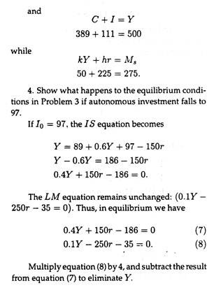
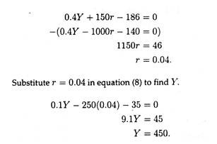
A fall in autonomous investment, ceteris paribus, will lead to a decrease in the equilibrium level of in­come and a drop in the interest rate.