Simultaneous Equilibrium of Goods Market and Money Market

Simultaneous Equilibrium of Goods Market and Money Market!

The IS and the LM curves relate the two variables.

(a) Income and

(b) The rate of interest.

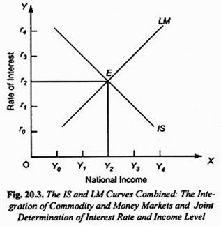
Income and the rate of interest are therefore determined together at the point of intersection of these two curves, i.e., E in Fig. 20.3. The equilibrium rate of interest thus determined is Or₂ and the level of income determined is OY₂.

At this point income and the rate of interest stand in relation to each other such that (1) the goods market is in equilibrium, that is, the aggregate demand equals the level of aggregate output, and (2) the demand for money is in equilibrium with the supply of money (i.e., the desired amount of money is equal to the actual supply of money). It should be noted that LM curve has been drawn by keeping the supply of money fixed.

Thus, the IS-LM curve model is based on:

(1) The investment-demand function,

(2) The consumption function,

(3) The money demand function, and

(4) The quantity of money.

We see, therefore, that according to the IS-LM curve model both the real factors, namely, saving and investment, productivity of capital and propensity to consume and save, and the monetary factors, that is, the demand for money (liquidity preference) and supply of money play a part in the joint determination of the rate of interest and the level of income.

Any change in these factors will cause a shift in IS or LM curve and will therefore change the equilibrium levels of the rate of interest and income. The IS-LM curve model explained above has succeeded in integrating the theory of money with the theory of income determination. And by doing so, as we shall see below, it has succeeded in synthesizing the monetary and fiscal policies.

Further, with the IS-LM curve analysis, we are better able to explain the effect of changes in certain important economic variables such as desire to save, the supply of money, investment, demand for money on the rate of interest and level of income.

Effect of Changes in Supply of Money on the Rate of Interest and Income Level:

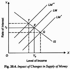
Let us first consider what will happen if the supply of money is increased by the action of the Central Bank. Given the liquidity preference schedule, with the increase in the supply of money, more money will be available for speculative motive at a given level of income which will cause the interest rate to fall.

As a result, the LM curve will shift to the right. With this rightward shift in the LM curve, in the new equilibrium position, rate of interest will be lower and the level of income greater than at point E. With the increase in the supply of money, LM curve shifts to the right to the position LM’, and with IS schedule remaining unchanged, new equilibrium is at point G corresponding to which rate of interest is lower and level of income greater than at E.

Now, suppose that instead of increasing the supply of money, Central Bank of the country takes steps to reduce the supply of money. With the reduction in the supply of money, less money will be available for speculative motive at each level of income and, as a result, the LM curve will shift to the left of E, and the is curve remaining unchanged, in the new equilibrium position (as shown by point T in Fig. 20.4) the rate of interest will be higher and the level of income smaller than before.

Changes in the Desire to Save or Propensity to Consume:

Let us consider what happens to the rate of interest when desire to save or, in other words, propensity to consume changes. When people’s desire to save falls, that is, when propensity to consume rises, the aggregate demand curve will shift upward and, therefore, level of national income will rise at each rate of interest.

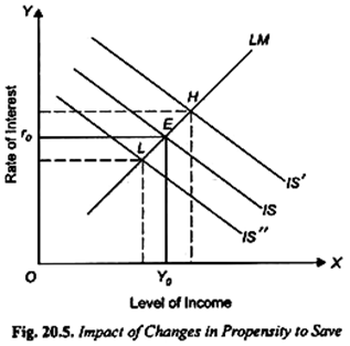
As a result, the IS curve will shift outward to the right. In Fig. 20.5 suppose with a certain given fall in the desire to save (or increase in the propensity to consume), the IS curve shifts rightward to the dotted position IS”. With LM curve remaining unchanged, the new equilibrium position will be established at H corresponding to which rate of interest as well as level of income will be greater than at E.

Thus, a fall in the desire to save has led to the increase in both rate of interest and level of income. On the other hand, if the desire to save rises, that is, if the propensity to consume falls, aggregate demand curve will shift downward which will cause the level of national income to fall for each rate of interest and as a result the IS curve will shift to the left.

With this, and LM curve remaining unchanged, the new equilibrium position will be reached to the left of E, say at point L (as shown in Fig. 20.5) corresponding to which both rate of interest and level of national income will be smaller than at E.

Changes in Autonomous Investment and Government Expenditure:

Changes in autonomous investment and Government expenditure will also shift the 75 curve. If either there is increase in autonomous private investment or Government steps up its expenditure, aggregate demand for goods will increase and this will bring about increase in national income through the multiplier process.

This will shift IS schedule to the right, and given the LM curve, the rate of interest as well as the level of income will rise. On the contrary, if somehow private investment expenditure falls or the Government reduces its expenditure, the IS curve will shift to the left and, given the LM curve, both the rate of interest and the level of income will fall.

Changes in Demand for Money or Liquidity Preference:

Changes in liquidity preference will bring about changes in the LM curve. If the liquidity preference or demand for money of the people rises, the LM curve will shift to the left. This is because, greater demand for money, given the supply of money, will raise the rate of interest corresponding to each level of national income. With the leftward shift in the LM curve, given the IS curve, the equilibrium rate of interest will rise and the level of national income will fall.

On the contrary, if the demand for money or liquidity preference of the people falls, the LM curve will shift to the right. This is because, given the supply of money, the rightward shift in the money demand curve means that corresponding to each level of income there will be lower rate of interest. With rightward shift in the LM curve, given the IS curve, the equilibrium level of rate of interest will fall and the equilibrium level of national income will increase.

We thus see that changes in propensity to consume (or desire to save), autonomous investment or Government expenditure, the supply of money and the demand for money will cause shifts in either IS or LM curve and will thereby bring about changes in the rate of interest as well as in national income.

The integration of goods market and money market in the IS-LM curve model clearly shows that Government can influence the economic activity or the level of national income through monetary and fiscal measures.

Through adopting an appropriate monetary policy (i.e., changing the supply of money) the Government can shift the LM curve and through pursuing an appropriate fiscal policy (expenditure and taxation policy) the Government can shift the IS curve. Thus both monetary and fiscal policies can play a useful role in regulating the level of economic activity in the country.

A Critique of the IS-LM Curve Model:

The IS-LM curve model makes a significant advance in explaining the simultaneous determination of the rate of interest and the level of national income. It represents a more general, inclusive and realistic approach to the determination of interest rate and level of income.

Further, the IS-LM model succeeds in integrating and synthesizing fiscal with monetary policies, and theory of income determination with the theory of money. But the IS-LM curve model is not without limitations. Firstly, it is based on the assumption that the rate of interest is quite flexible, that is, free to vary and not rigidly fixed by the Central Bank of a country.

If the rate of interest is quite inflexible, then the appropriate adjustment explained above will not take place. Secondly, the model is also based upon the assumption that investment is interest-elastic, that is, investment varies with the rate of interest. If investment is interest-inelastic, then the IS-LM curve model breaks down since the required adjustments do not occur.

Thirdly, Don Patinkin and Milton Friedman have criticized the IS-LM curve model as being too artificial and over-simplified. In their view, division of the economy into two sectors – monetary and real – is artificial and unrealistic. According to them, monetary and real sectors are quite interwoven and act and react on each other.

Further, Patinkin has pointed out that the IS-LM curve model has ignored the possibility of changes in the price level of commodities. According to him, the various economic variables such as supply of money, propensity to consume or save, investment and the demand for money not only influence the rate of interest and the level of national income but also the prices of commodities and services.

Patinkin has suggested a more integrated and general equilibrium approach which involves the simultaneous determination of not only the rate of interest and the level of income but also of the prices of commodities and services.