In this article we will discuss about:- 1. Demand for Money 2. Relation between the Rate of Interest and the Price of Bonds 3. Relation between the Rate of Interest (r) and the Speculative Demand for Money (L2) 4. Demand for Money in Aggregate 5. Supply of Money 6. Determination of the Equilibrium Rate of Interest 7. Critical Evaluation.
Contents:
- Demand for Money
- Relation between the Rate of Interest and the Price of Bonds
- Relation between the Rate of Interest (r) and the Speculative Demand for Money (L2)
- Demand for Money in Aggregate
- Supply of Money
- Determination of the Equilibrium Rate of Interest
- Critical Evaluation of the Keynesian Liquidity Preference Theory
1. Demand for Money:
Demand for money means the willingness of the households and the businesses to hold liquid money. Keynes has called the demand for liquid money the liquidity preference.
ADVERTISEMENTS:
According to Keynes, the households and the businesses are willing to hold money for three purposes or motives.
These are:
(i) Transactions motive,
(ii) Precautionary motive, and
ADVERTISEMENTS:
(iii) Speculative motive.
Transactions Demand for Money:
People (the households and businesses) are willing to hold some amount of money for daily transactions. For a person does not spend all his income as soon as he receives it. For example, a consumer’s spending of the money he receives as income in the beginning of the month, is spread all over the month.
ADVERTISEMENTS:
The firms also hold money for transactions purposes. Generally, they do not spend for transactions purposes, e.g., for buying raw materials or making payments to workers as soon as they receive their sales proceeds. The willingness to hold money for transactions purposes is known as transactions demand for money.
Now, how much money a household or a businessman is to hold on average for making transactions, will depend on his income. The more the income, the more would be the demand for money for transactions purposes. That is why the transactions demand for money in aggregate in a country depends upon the national income.
Precautionary Demand for Money:
The households and businesses of a country are willing to hold some amount of money for contingencies. For example, a person may fall victim to accidents, illness, unemployment and such other crises. Emergency may arise in businesses also.
The willingness of the people to hold money as precautions against such uncertainties is called the demand for money for precautionary purposes. This demand for money, like the transactions demand for money, also depends upon the country’s level of income.
Demand for Active Balance:
The money the people hold for transactions and precautionary purposes taken together is called active balances. For, this money is held for active spending.
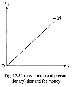
On the whole, the demand for active balances depends upon the country’s level of income, for both the components (the transactions and precautionary) of this demand directly depend upon income. The higher the level of income, the more would be this demand. If we denote the demand for active balances by L1, then we may write
L1 = L1(y), L’1 > 0 (17.8)
ADVERTISEMENTS:
where L1 = demand for money in real terms for transactions and precautionary purposes and
y = real income.
If we assume that the relation between y and L1 is linear, then this relation may be represented by the straight line, L1 (y), in Fig. 17.3. This line would start from the point of origin, O, for theoretically, L1 = 0 at y = 0. Again, the slope of the line would be positive, for L1 increases as y increases. We can know from this line the value of L1 at any particular value of y.
ADVERTISEMENTS:
Speculative Demand for Money:
The buying and selling of goods with a view to earning profit, on the basis of guess about the changes in price in future, is known as speculative activity. Keynes has discussed in his liquidity preference theory about speculative business in bonds or securities. He has said that when the price of bonds falls, people buy more bonds, and when the price rises, people increase their sale of bonds.
ADVERTISEMENTS:
They generally hold money they receive from selling the bonds. They buy bonds with this money when the bond prices fall. The holding of money by the people to continue with the speculative business is called the speculative demand for money. We denote this demand by L2.
2. Relation between the Rate of Interest and the Price of Bonds:
Speculative demand for money (L2) depends upon the rate of interest (r). To understand this, we have to understand first the relation between r and the bond price (pb).
A bond or security is a certified paper. The government of a country may issue bonds apparently to borrow money.
On the face of the bond paper are mentioned:
(i) The issue price or the face value of the bond, e.g., Rs. 100; and
ADVERTISEMENTS:
(ii) The yield per year of the bond which is also called coupon, e.g., Rs 10 = constant, or, in this case, 10 per cent (of the face value).
Now, if a need for cash arises, the owner of the bond may sell it in the bond market. Let us suppose, when he decides to sell the bond, the rate of interest has declined to 5 per cent. So now he would be able to sell the bond at a price of Rs 200, which is called the market price of the bond.
For, now (at 5 per cent), the yield of a newly issued bond of face value of Rs 100 is Rs 5 per year and to obtain a yield of Rs 10 a person has to buy new bonds worth face value of Rs 200. Therefore, the old bond of face value of Rs 100 and yield of Rs 10 would now fetch a price of Rs 200 in the market. For the old bond, the face value is Rs 100 and the market price now is Rs 200.
Again, if the rate of interest is 20 per cent when the person decides to sell the bond, he would get only Rs 50 as the market price of the bond. Because, now, at r = 20 per cent, Rs 50 worth of newly issued bonds would have a yield of Rs 10.
As we have seen in the above example, as r falls from 10 per cent to 5 per cent, the market value of the bond rises from Rs 100 (which is initially the face value = market value) to Rs 200, and if r rises from 10 per cent to 20 per cent, the market value of the bond falls from Rs 100 to Rs 50.
That is, as r declines, the (market) price of bonds rises and, as r rises, the (market) price of bonds falls, i.e., r and the bond price are inversely related. Also, in our example, we see that as r is halved, the bond price is doubled and as r is doubled, the bond price is halved. That is, r and the bond price (pb,) are not only inversely related, but their relation is inversely proportional also.
ADVERTISEMENTS:
ADVERTISEMENTS:
3. Relation between the Rate of Interest (r) and the Speculative Demand for Money (L2):
We may now easily determine the nature of the relation between rate of interest (r) and speculative demand for money (L2). For, as we know now, if r rises, the price of bonds will fall and consequently, the speculators will increase their demand for and purchase of bonds, to sell them eventually at higher prices.
Now, if they increase the purchase of bonds with their speculative balance, then speculative money holding (L2) will fall.
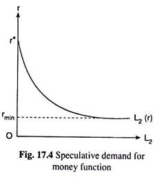
That is, if r rises, L2 will fall. On the other hand, if r falls, price of bonds will rise and this will make the speculators increase their sale of bonds to make profit out of the price rise, and consequently, their speculative balance will rise. That is, if r falls, L2 will rise. This relation between r and L2 is represented by the speculative demand for money [L2 (r)] curve in Fig. 17.4.
It is clear from the above analysis that there is, in general, an inverse relation between r and L2. We may express, therefore, the macro real demand for speculative balances (L2) as
ADVERTISEMENTS:
L2=L2(r), L’2<0 (17.9)
Exceptions to the General Relation between r and L2:
Although, ordinarily, the relation between r and L2 is inverse, there are two important exceptions to this general relation. First, as r decreases, some people may think at any particular point that r will no more decrease, i.e., price of bonds (pb) will no more increase.
Therefore, they will now sell all their bonds. Again, there may be some other people who may think that r will still go on falling and pb will go on rising. Therefore, they will, if at all, sell some, not all, of their bonds now, and keep the rest of their bonds for selling at an opportune moment in future.
However, r may ultimately fall to such a low and pb may rise to such a high that all the speculators may think alike—all of them may think at the same time that r cannot fall further and pb cannot rise further; on the contrary, now, r would start rising and pb would start falling.
In these circumstances, none of the speculators would be willing to buy bonds any more, rather, all of them would be willing to sell all their bonds. Owing to such behaviour of the speculators, pb cannot rise really and r cannot fall. Therefore, at the said ‘low’ r, the supply of bonds would be indefinitely large and the demand for speculative balances also would be indefinitely large.
ADVERTISEMENTS:
That is why, at this r, the L2 curve would be a horizontal straight line as shown in Fig. 17.4. In this Figure, we see that so long as r > rmin, L2 will rise as r falls, i.e., the curve would be sloping downwards towards right, and at r = rmin, the L2 curve would be a horizontal straight line. This horizontal segment of the L2 curve is called the special Keynesian range or the liquidity trap zone.
The second exception to the generally inverse relation between r and L2 is this. As r rises and pb, falls, the speculators would go on purchasing bonds from the market, and consequently, their bond holding increases and speculative demand for money decreases till r rises to such a high level and pb, falls to such a low level that the speculative balances with the traders in bonds become zero (L2 = 0), since by this time they have spent all their balances for buying bonds. If r rises further beyond this level of r = r*, say, then also L2 would remain equal to zero.
Therefore, in Fig. 17.4, at r ≥ r*, we obtain L2 = 0, and the L2 curve would become a vertical straight line, and it would coincide with the vertical (r) axis. Along this vertical segment of the L2 curve, speculative demand for money would be zero—demand for money now would only be for transactions and precautionary purposes—it would be only L1.
Since, to the classical economists, demand for money was only L1, the vertical segment of the L2 curve, (with L2 = 0), is called the classical range.
In the above analysis, we have seen that the L2 curve generally would be a negatively sloped curve. But it would have a vertical segment at the beginning and a horizontal segment towards the end. The negatively sloped segment of the L2 curve between the above two segments is called the intermediate range.
4. Demand for Money in Aggregate:
There are three motives, viz., transactions, precautionary, and speculative, behind the demand for money. The total demand for money owing to these motives is called the aggregate demand for money or the liquidity preference. If we denote this demand by L, then we may write
L = L1 (y) + L2 (r) = L(y, r); ∂L/∂r > 0, ∂L/∂r < 0 (17.10)
That is, the demand for money or liquidity preference, L, is a function of y and r. For, the L1 part of L is a function of income (y), and the L2 part is a function of r. If y increases, r remaining constant, then L1 would increase, and so, L would increase. That is why we obtain ∂L/∂y > 0.
Again, if r increases, y remaining constant, then L2 would fall, and so, L would fall. That is why we would have ∂L/∂r < 0.
Now, if we assume that y remains unchanged at a particular level, say, y̅, then L1 also would remain unchanged at the level, L1 (y̅).
In this case, we would obtain from (17.10):
L = L1(y) + L2(r) = L(r), L’ < 0 (17.11)
From (17.11) we obtain, since L1 = constant, that, as r rises (or falls), L2 falls (or rises) and L also falls (or rises). That is, the demand for money or liquidity preference (L) has been obtained to be an inverse function of the rate of interest (r).
We also obtain from (17.11) that we would know L if we add L1 (= constant) to L2 (r). We have shown such an L curve in Fig. 17.5. Here we have supposed, L1 (y̅) = OA. As we have said above, L2, and therefore, L2 + OA = L also, is indefinitely large at r = rmin. That is, at r = rmin, the L curve also, like the L2 curve, would be a horizontal straight line.
The horizontal segment of the L curve, like that of the L2 curve, is also called the special Keynesian range or the liquidity trap zone. Again, for r > r*, we have L2 = 0 and so we would have: L = L2 + OA = OA = L1 = constant. That is, for r ≥ r*, the L curve like the L2 curve would be a vertical straight line.
This vertical segment of the L curve, like that of the L2 curve, is known as the classical range. For, when r rises to a certain level or beyond that (here r ≥ r*), demand for money (L) is composed of only L1 (L2 = 0), as the classical economists thought.
The negatively sloped segment of the L curve between its vertical and horizontal segments, like that of the L2 curve, is called its intermediate range. We have to note here that the L curve would be vertical and horizontal at the same rates of interest at which the L2 curve happens to be vertical and horizontal (here at r = r* and rmin), respectively. At any rate of interest that falls between these two rates (r* and rmin), the L2 and L curves both would be negatively sloped.
5. Supply of Money:
Keynes has analysed demand for money in sufficient details. But in his theory, matters regarding supply of money have not been discussed in that way. Keynes has said that the monetary authorities (government and central bank) determine the supply of money, and this supply is controlled according to the monetary policy of the authorities.
Without going into the discussion of the determinants of this policy Keynes has assumed that the nominal supply of money (M) at any point in time would be exogenously given by the monetary authorities of the country. In other words, in Keynes’ theory, the supply of money has been assumed to be an exogenously given parameter. If we denote the supply of money in real terms by m, then we may write
m = M̅/P0 = m̅ = constant (17.12)
where M̅ = the given value of M = constant
and P0 = the prevailing price level of the country = constant.
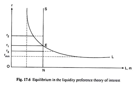
Since the supply of money has been assumed here to be a constant independent of the rate of interest (r), we have drawn the supply of money curve in Fig. 17.6 as a vertical straight line. In this figure, we have m̅ = ON = constant at any r.
6. Determination of the Equilibrium Rate of Interest:
Following Keynes, we may easily determine the equilibrium rate of interest in his theory. For, it is the rate at which the demand for and supply of money become equal to each other. In Fig. 17.6, the demand for money and supply of money curves are, respectively, L and NS.
Here the equilibrium rate of interest has been r = r1, which has been obtained at the point of intersection E between the L and NS curves. At this rate of interest, i.e., at r = r1, the demand for money has become equal to the (exogenously given) supply of money.
Since demand for money and supply of money are equal at r = r1, nobody on the demand side or the supply side of the money market would be interested in changing this r. That is why this r = r1 is the equilibrium rate.
From the above analysis, it is obtained that in Keynes’ liquidity preference theory of interest, the condition for equilibrium r or for equilibrium in the money market is
L(r) = m̅ (17.13)
where L(r) is the demand for money and m̅ is the exogenously given supply of money, both in real terms.
This Equilibrium is a Stable Equilibrium:
We may now see why any r other than r, in Fig. 17.6 cannot be accepted as the equilibrium r. Let us suppose, r = r2 > r1. Then demand for money (L) would be smaller than the supply of money (in). That is, the households and the businesses are demanding (willing to hold) less money than the amount of money (supply of money) lying with them, i.e., they are wanting a change of the present situation in respect of money holding.
That is why we may say that there is no equilibrium in the money market. Under the circumstances, they would want to get rid of some of the money they are holding at present, i.e., they would want to buy bonds with their excess money holding.
As a consequence of this, demand for bonds and the price of bonds will rise and the rate of interest (r) will fall. As r falls, demand for money (L) will rise. When r has fallen to the level of r = r1 and demand for money has increased to L = ON = m̅, equilibrium will be restored in the money market. For now, there would be no tendency for r to change. That is why, r = r1 is the equilibrium rate of interest.
On the other hand, if r = r3 < r1, then demand for money (L) would be greater than the supply of money (m̅). That is, here the households and businesses are demanding more money than the supply of money lying with them, i.e., here also they are wanting a change of the present situation in respect of money holding. Therefore, there is no equilibrium in the money market.
Under the circumstances they would seek to have more money than they are holding at present, i.e., they would be willing to sell some of the bonds held by them to meet their excess demand for money.
As a consequence, supply of bonds will rise and the price of bonds will fall leading to a rise in the rate of interest (r). As r rises, demand for money (L) will fall. When r has risen to the level r = r1, and demand for money has decreased to L = ON = m̅, equilibrium will be restored in the money market.
Therefore, we have obtained in the above analysis that if the rate of interest and the money market are not in equilibrium, then people (households and businesses) will behave (will buy or sell bonds) in such a way that the market will again come back to equilibrium. That is why this equilibrium is a stable equilibrium.
Conditions for Stability of Equilibrium in the Money Market:
We may now mention briefly the conditions for stability of equilibrium in the money market. The assumptions about the behaviour of the households and the businesses that we have made in the preceding section are: If L < m̅, they will increase their demand for bonds. Consequently, the price of bonds will rise and r will fall.
Again, if L > m̅, they will increase their supply of bonds. Consequently, price of bonds will fall and r will rise. Subject to these assumptions, the conditions for stability of equilibrium in the money market are: If the rate of interest (r) be greater than the equilibrium rate (re), then L would be less than m̅, and, if r < re, then L would be greater than m.
If the demand curve (L) for money is downward sloping and the supply of money (m̅) curve is upward sloping or a vertical straight line, then these conditions for stability of equilibrium will be satisfied. Since, in the liquidity preference theory, the L curve is ordinarily negatively sloped and the m̅ curve is a vertical straight line, the money market equilibrium in the theory as shown in Fig. 17.6 is a stable equilibrium.
Effects of a Rise in the Demand for and Supply of Money on the Rate of Interest:
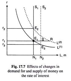
Let us suppose that the demand and supply curves for money are the curves L(1) and N1S1, respectively, in Fig. 17.7. Here the equilibrium rate of interest is r1 at the point of intersection E1 of these two curves.
If, now demand for money increases, the supply of money remaining unchanged, the L curve would shift to the right from L(1) to L(2), say. Consequently, at r = r1, the demand for money would be larger than the supply of money by E1R.
In this case, r will rise and L will fall along the RE1 segment of the L(2) curve, till demand for money becomes equal to supply at the point E2. In Fig. 17.7, when r will rise from r1 to r2, the equilibrium in the market would again occur at the point E2 which is the point of intersection of the L(2) and N,S, curves.
Therefore, if the demand for money increases, the supply remaining unchanged, then the equilibrium r will rise. On the other hand, if demand falls supply remaining unchanged, i.e., if the demand for money (L) curve shifts to the left, the position of the supply curve remaining unchanged, then the equilibrium r will fall. That is, r is directly related to L.
Again, if the supply of money increases, demand remaining unchanged, then the supply of money curve would shift to the right from N1S1 to N2S2, the position of the demand curve remaining unchanged at L(1).
Consequently, at the initial equilibrium r = r1, the supply of money would be greater than demand for money by E1S. In this case, r will fall and L will rise along E1E3 segment of the L(1) curve till the demand for money (L) becomes equal to supply (ON2) at the point E3.
In Fig. 17.7, the market will again come back to equilibrium at the point E3 when r falls from r, to r3. E3 is the point of intersection of the L(1) and N2S2 curves.
Therefore, that if the supply of money increases, demand for money remaining unchanged, then the equilibrium r will fall. On the other hand, we may also see, that if the supply of money falls, demand remaining unchanged, i.e., if the supply of money (in) curve shifts to left, the position of the demand curve remaining unchanged, then the equilibrium r will rise. That is, r is inversely related to m̅.
Here we have also seen that whenever the money market moves away from equilibrium owing to a change in the demand for, or, supply of money, the rate of interest and demand for money change in the opposite directions of each other to bring the market back to equilibrium (supply of money being exogenously given).
This implies that here the L curve has been assumed to be negatively sloped, neither horizontal nor vertical.
The Liquidity Trap:
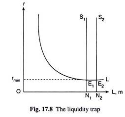
While discussing the effects of a change in the supply of money on the rate of interest, we have to note that if the change occurs over the horizontal segment of the liquidity preference (L) curve, then it would have no effect on the rate of interest. In Fig. 17.8, the L curve is the demand curve for money or liquidity preference curve and the N1S1 line is the supply curve of money.
Since the market equilibrium point E1 lies on the horizontal segment of the L curve, the equilibrium r is rmin. Now if the supply of money rises from ON1 to ON2, i.e., if the supply curve of money shifts to the right from N1S1 to N2S2 over the horizontal segment of the L curve, then the demand for money and supply of money would be equal and the market would be in equilibrium at the point E2 at the same rmin.
For here, in spite of an increase in the supply of money, people will not go to use the money to buy bonds. For, now everybody thinks that r would not fall below rmin and the bond price is not going to rise above its present level. On the contrary, sooner or later, r will rise and the price of bonds will fall.
Therefore, if bonds are purchased now, then the buyers of bonds will suffer a capital loss. Under the circumstances, even if the supply of money or liquidity increases, demand for bonds and the price of bonds will not increase, and so, r will not fall. Such a situation is known as liquidity trap.
7. Critical Evaluation of the Keynesian Liquidity Preference Theory:
Keynes in his theory of interest has correctly put emphasis on the demand for and supply of liquid assets and money. However, like the classical and neoclassical (loanable funds) theories of interest, Keynes’ theory is not without defects.
The defects of this theory are:
(i) The theory considers only the monetary factors like the demand for and supply of money. It has not recognised the fact that, along with the monetary factors, the real factors like the marginal productivity of capital and the propensity to save may also influence the rate of interest.
But this is only apparently. If we think a little more deeply, we would find that the businessmen’s demand for money for transactions purposes is influenced by the investment demand for (money) capital—the more the investment demand for money, the more would be their transactions demand for money.
The investment demand for capital, again, depends upon the real factors like the marginal productivity (MP) or the marginal efficiency (ME) of capital. If there are bright prospects for earning profit, the MP or ME of capital will increase and, as a result of this, the demand for money of the businesses and the rate of interest will rise.
Similarly, there is no mention in Keynes’ theory that the propensity to save might also influence the rate of interest (r). But we have to remember that if the propensity to consume of the people increases and the propensity to save decreases, then the transactions demand for money increases on the one hand, and, on the other hand, the supply of bonds would increase (more bonds would be sold) to meet this demand and, consequently, the price of bonds decreases and the rate of interest increases.
Therefore, in Keynes’ theory also, the real factors like the productivity of capital, the propensities to consume and save influence the rate of interest, at least indirectly, if not directly.
(ii) Like the classical and the neoclassical theories of interest, Keynes’ liquidity preference theory of interest is also indeterminate. For here also, to know the demand for money, viz., L = L1 (y̅) + L2 (r), at different rates of interest, we have to know L) (y̅), and to know L1 (y̅), we have to know y or the (equilibrium) level of income of the country which has been assumed to be fixed at y. Again, to know y, we have to know the country’s level of investment, i, because y̅ (via multiplier) depends upon i. Again, to know i, we have to know r, since i = i (r), i'<0.
Therefore, it is clear from the above arguments that to determine r, we have to know r beforehand. That is why, Keynes’ liquidity preference theory cannot determine the rate of interest.
(iii) If a person buys bonds in exchange of liquid money, he gets interest, but he has to lose liquidity. According to Keynes, interest is a reward for being deprived of liquidity, it is not a reward for savings or for being deprived of present consumption.
But here we have to remember that a person may be an owner of liquid assets only by means of savings. Therefore, being deprived of liquidity implies being deprived of one’s savings, and to regard interest as a reward for losing liquidity means to regard interest as a reward for being deprived of savings.
Two things are clear to us from the above discussion. First, in the Keynesian theory of interest, the real factors like propensity to save, productivity or efficiency of capital, suffering for abstaining from present consumption, etc., have an important role to play at least indirectly. Second, the theory of Keynes, like the classical and neoclassical theory, is indeterminate—the theory cannot determine a unique rate of interest.
