Beginners Guide to Keynesian Model

Beginners Guide to Keynesian Model!

The Keynesian System:

The theoretical scheme of the classical/neo-classical economists describes the self-equilibrating character of competitive capitalism, but failed to explain the long depression of the 1930s.

Economists and policy-makers became sceptical about the classical postulates. As a result, a new macroeconomic system was developed in the publication of the General Theory of Employment, Interest and Money by J. M. Keynes which is known as the Keynesian Macroeconomics. Thus, Keynesian system is the core of modern macroeconomic theory.

The Keynesian system gives an alternative set of postulates and establishes the case of an under-employment equilibrium. In the Keynesian system, involuntary unemployment can exist if part of work-force do not get jobs even when they are willing to work at the existing money wage rate because of the absence of job opportunities.

The existence of involuntary unemployment makes the economy attain equilibrium before full employment is reached. It is the theoretical possibility of the under-employment equilibrium which is the most striking departure of the Keynesian system from the classical system.

Another feature of the Keynesian system which makes it different from the classical system is the interdependence among all macroeconomic variables. In this system, real income, rate of interest, price level, employment and real wages are all determined simultaneously.

As we have seen, in the simple Keynesian model of income determination, the equilibrium level of income is determined by the equality of planned saving and planned investment (or by the equality of aggregate demand and aggregate supply). Saving is a function of income and investment is a function of interest rate.

Thus, in the market for commodities, we write the following three equations:

1) S = S(Y) — Saving function

2) I = I(r) — Investment function

3) S = I — Equilibrium condition

The system is indeterminate because this model has three equations and four unknown variables (S, I, r and Y). Since investment is a function of the rate of interest, we cannot determine the equilibrium level of income from the equations of the commodity market. Unless we know the equilibrium rate of interest we cannot know the equilibrium level of income.

From the equilibrium condition in the commodity market we can get the different combinations of r and Y for which saving will be equal to investment. All these combinations of Y and r give the IS curve. To determine the interest rate we turn to the liquidity preference theory of interest rate determination.

In this theory also, there are three money market equations which are given below:

(4) M_D = M_t + L(r) = KPY + L(r) → money demand function

(5) M = M₀ → money supply function

(6) M_D = M → equilibrium condition

In the money market also there are three equations and four unknowns – L, M, r and Y. Hence we can only determine the value of r when we know the value of Y. From the equilibrium condition in the money market, we can find different combinations of r and Y. The locus of all such points gives the LM curve.

We have seen that we cannot determine the equilibrium level of income from equations of the commodity market alone. Similarly, it is also not possible to determine the rate of interest from the equations of the money market alone Equilibrium level of income depends on the interest rate and the equilibrium rate of interest also depends on the level of income. One cannot be determined without the other.

There is interdependence between the commodity market and the money market. Thus, equilibrium income and interest rate are determined simultaneously. Since the equilibrium in both the markets have to be achieved simultaneously, we can get general equilibrium.

In order to develop the Keynesian system, we need to bring together the six functional relations. The consumption function (or the saving function), the investment function, the demand for money function, the aggregate production, the demand and the supply function of labour. Of these six functional relations, three are the same as in the classical system and the other three are significantly different from the classical forms.

The investment function, the aggregate production function and the demand function for labour are based on the same postulates in the Keynesian and classical system. But the other three functions, the saving function — the demand function for money and the supply function for labour— are significantly different from the classical system.

We discuss first the commodity and the money market relations to determine the equilibrium level of income and the equilibrium interest rate simultaneously. In the system so far developed, there are six equations and six unknown variables. Thus, the system of equations can be solved.

The equations (1) – (3) can be written as a single equation:

(3′) S(Y) = I(Y) — Equation of the IS curve

Similarly, equations (4) – (6) can be expressed as a single equation:

The equation of the LM curve – (6′) M₀ = KPY +L (Y)

The system of six equations can be transformed into a system of two equations and two unknowns – rand Y. Equations (3′) and (6’) are simultaneous equations which can be solved to get the equilibrium values of r and Y.

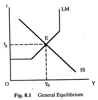
The IS curve gives us different combinations of r and Y for (S will be equal to I) which the commodity market would be in equilibrium. This curve is normally downward sloping. The LM curve will give us different combinations of r and Y for which the money market would be in equilibrium (M_d = M₀). The LM curve as before will have horizontal range upward rising and vertical range.

We bring the IS and LM curves in a single diagram (Fig. 8.1) These two curves intersect at E where both the equilibrium conditions arc fulfilled (i.e., IS = LM) At point E. the equilibrium level of income Y₀ and the equilibrium rate of interest r₀ are achieved. When IS curve is downward sloping and the LM curve is upward rising they can intersect once only. Hence the equilibrium is unique.

Stability Condition of the Equilibrium:

If the slope of IS curve minus the slope of the LM curve is negative, then the equilibrium can be said to be stable. Since the IS curve is normally negatively sloped and the LM curve is positively sloped the stability condition is automatically fulfilled. However, if the IS curve is positively sloped, then the stability condition can only be satisfied if its slope is less than the LM curve. This requires the IS curve to cut the LM curve from above. Otherwise the equilibrium would be unstable.

Alternatively, the stability con­dition can be analysed by assuming the dynamic adjustment in commod­ity and money markets work in such a way that whenever there is an excess demand or excess supply, the rate of interest and the level of income will change.

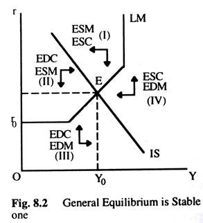
Or if we assume that the rate of interest will decrease (increase) if there is an excess supply (demand) in the money market and the level of income will increase (decrease) if there is an excess demand (supply) in the commodity market. The stability can be proved with the help of the diagram given (Fig. 8.2). Suppose that the IS and LM curves intersect to produce four regions in Fig. 8.2.

In region I, there is excess supply in the commodity market (ESC) and excess supply in the money market (ESM). Thus, both income (Y) and interest rate (r) will fall as shown by the arrows. In region I – there is ESC i.e. Y↓ ESM i.e. r↓. In region II, there is excess demand in the commodity market (EDC) and excess supply in the money (ESM).

Thus, the level of income (Y) will rise and the interest rate will as the arrows show. In region II – EDC i.e. Y↑ ESM i.e. r↓. In region III, there is excess demand in the commodity market (EDC) and excess demand in the money market (EDM). The result would be that both the level of income and the rate of interest will increase. This can be shown as in region III – (EDC) i.e. Y↑ and also (EDM) i.e. r↑.

In the same way, the movements of r and Y in region IV can be shown as follows:

In region IV – (ESC) i.e. Y↓ and (EDM) i.e. r↑. It can now be shown that if we start from any other point than the point of intersection between the IS and the LM curves the market forces will work to bring the level of income and the rate of interest to the point of intersection of the IS and the LM curves at E.

The different market forces affecting r and Y in different regions are shown by the direction of arrows in Fig. 8.2. For example, in region I, arrows indicate that both r and Y will fall because there is excess supply in both the commodity and money markets.

As a result of their fall, we can either directly approach the equilibrium point E or can enter the region where market forces will again be generated to push r and Y either towards E or to region III and so on. The market forces will continue to work until the equilibrium point E is reached. Thus, from whatever point we start with, we shall end up at the equilibrium point E. Therefore, the equilibrium is a stable equilibrium.

Effect of Change in Money Supply on the Equilibrium Rate of Interest and Income with Fixed Price Level:

We know that the equilibrium level of income and interest rate are determined by the intersection of IS and LM curves. We derived the LM curve on the assumption that the money supply and the price level are given. Thus, when the money supply changes the price level being given, the LM curve will shift while the IS curve will remain unaffected.

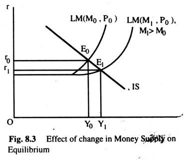
Hence, the equilibrium rate of interest and income will be affected when the money supply changes. When the money supply increases with the price level remaining unchanged, the LM curve shifts to the right. The effect of this shift on the equilibrium level of income and interest rate can be seen in Fig. 8.3. Suppose that, at the initial equilibrium, price is P₀, where the level of income is Y₀, and the Interest rate is r₀.

Now, money supply increases from M₀ to M₁, the LM curve shifts to the right and the new equilibrium point moves from E₀ to E₁ — where income is Y₁ and the rate of interest is r₁. Since r₁ < r₀ and Y₁ > Y₀, we can say that the effect of an increase in money supply is to increase the equilibrium level of income (from Y₀ to Y₁) and to reduce the interest rate (from r₀ to r₁).

Now we wish to discuss the mechanism through which these changes take place. As the supply of money increases, the demand for money remaining unchanged, a situation of excess supply is created in the money market which leads to a fall in the market rate of interest.

Alternatively, it can be said that, as money supply increases, a part of the additional money entered into the bond market increases the demand for bond leading to an upward movement in the price of bonds. An increase in the price of bonds means a fall in the interest rate. We also know that there is an inverse relationship between investment and the rate of interest. Thus, as the rate of interest falls, investment increases which increases the level of income through the usual multiplier effect.

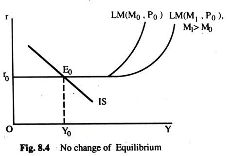
There are two exceptions to this general rule. In the first case suppose that the IS curve intersects the LM curve at the LM curve’s horizontal position. This is shown in Fig. 8.4. As money supply increases from M₀ to M₁, the LM curve shifts to the right hut the equilibrium point remains unchanged at E₀.

In this situation, the money demand function is perfectly interest-elastic and everyone prefers cash to bonds and no part of the new money supply will reach the bond market. As a consequence, bond prices will not rise and the interest rate will not fall. This is known as the liquidity trap situation where monetary policy becomes completely ineffective and the changes in money supply will have no effect on the level of income and the rate of interest as discussed earlier.

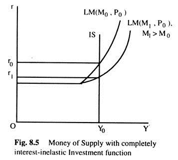
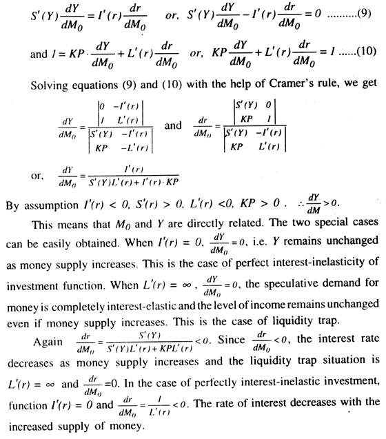
The second case arises when the investment function is completely interest-inelastic. In this case l'(r) = 0 and dr/dY = ∞. This means that IS curve is a vertical straight line. Thus, as money supply increases, the market rate of interest is reduced, but the level of income remains unchanged because the investment is perfectly interest-inelastic (i.e. the volume of investment do not change in response to change in the rate of interest). As investment remains unchanged the level of income also remains the same as shown in Fig. 8.5. The effect of change of money supply can be mathematically analysed as follows.

Two equilibrium conditions are given below:

(7) S(Y) = l(r) and (8) M₀ = KPY + L(r).

By differentiating the two equations with respect to M₀, we can see the effect of change in money supply on Y and r.

Investment Multiplier in the IS-LM Model:

Suppose the investment function is now written as:

I = l(r) + A

where A represents autonomous investment.

Thus, a change in A means a change in autonomous or exogenous investment expenditure. Now let us examine how the equilibrium level of income is affected when A changes in the IS-LM model.

There are two equations in the model:

(1) S(Y) = I(r) + A and (2) M₀ = KPY + L(r)

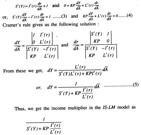
From the solution of these two simultaneous equations, we get the equilibrium values of Y and r. When A changes the equilibrium value of Y and r will also change which can be obtained by differentiating equations (1) and (2) with respect to A and solving for dY/dA and dr/dA.

By differentiating, we get the following result:

From our assumption that S'(Y) > 0, I'(r) < 0 and L'(r) < 0, the multiplier is positive which means that as A increases the equilibrium level of income also increases.

Thus, the multiplier in the IS-LM model is smaller than the multiplier in the simple Keynesian model as given below:

This is so because the investment in the IS-LM model is not completely autonomous. One part of the investment is a function of the rate of interest and the other part is autonomous. When the autonomous investment increases- the equilibrium level of income and the rate of interest also increases. An increase in the rate of interest decreases induced investment. Thus, the net increase in income is lower in this case when investment is also a function of the rate of interest.

However, there are two exceptional cases when the multiplier in the IS- LM model will be equal to the simple Keynesian multiplier 1/S’(Y). First, where the investment function is completely interest inelastic, the full multiplier effect is obtained i.e. the multiplier becomes 1/S’ (Y) when l'(r) = 0. Second, if the money demand function is absolutely interest elastic, then also full-multiplier effect can be obtained. When L'(r) → ∞, from dr/dA = -KP/S’ (Y) L’ (r) + KPI’ (r) we get dr/dA = 0. This means that the rate of interest does not rise when autonomous investment increases and induced investment also does not fall. Thus, the full multiplier effect is obtained.

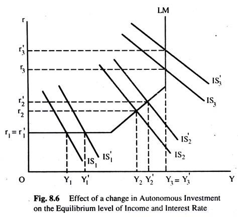
This can be explained with the help of Fig. 8.6. As autonomous investment increases the IS curve shifts to the right. Now the effect on the equilibrium level of income depends on where the IS curve intersects the LM curve. We can have three situations as the Fig. 8.6 shows.

First, suppose the IS curve intersects the LM curve at its horizontal part before and after the shift. When the IS shifts to IS₁, the level of income increases from Y₁ to Y₁, but the interest rate remains unchanged at r₁ = r₁ In this range, L'(r) => ∞ and the multiplier is equal to 1/S’ (Y).

Second, suppose the IS₂ curve shifts from IS₂ to IS₂ and intersects the LM curve at its rising part. Here the equilibrium level of income increases from Y₂ to Y’₂ and the interest rate increases from r₂ to r₂. In this range, the multiplier is equal to 1/S’ (Y) + KP I’(r)/L’(r). Third, now suppose that the IS curve intersects the LM curve at its vertical part both before and after the change. When IS curve shifts from IS₃ to IS₃, the equilibrium level of income remains the same and only the interest rate increases from r₃ to r’₃ where L'(r) = 0, dY/dA = 0, which means Y remains the same. From equation (5), we get dr/dA = I/I’ (r) >0, which means that the interest rate increases.

Limitation of the IS-LM Model:

The assumption behind the IS-LM model is that the price level is given as constant and the level of income is demand determined. The assumption of fixed price implies that the aggregate supply curve is perfectly elastic (a horizontal straight line).

This is true only if there is excess capacity in the economy so that extra output can be produced at constant marginal cost. If the supply curve is perfectly elastic only then the level of output can be determined by the position of the demand curve. In the IS-LM model, the equilibrium level of output is demand-determined. Such a situation seems unrealistic.

If the supply of output is not perfectly elastic, higher output can be produced only at a higher price. The price level is no longer constant in such a situation. If the price level varies with the output, the model becomes indeterminate since we have two equations and three unknowns – r, Y and P.

Alternatively, the LM curve is drawn on the assumption that the supply of money and the price level are fixed. Now, if the supply of money is still assumed to be fixed, the LM curve will shift as the price level changes. Thus, equilibrium level of income cannot be determined unless the equilibrium price level is known. The IS-LM model cannot help us to determine equilibrium price level.

Moreover, the IS-LM model considers only the goods and money markets. It does not consider the labour market at all. Without the labour market and the production function the level of output cannot be determined. It does not consider the supply side of the economy. It only considers the demand side. It gives only the aggregate demand curve but not the aggregate supply curve without which the equilibrium price level cannot be determined.

The Labour Market:

Unless the equilibrium price level is determined, we cannot find out the equilibrium level of income and interest rate. Let us see how the equilibrium price level is determined in the economy. In the labour market, we derive the labour demand and the labour supply functions. The labour demand function is derived from the aggregate production function as in the classical system.

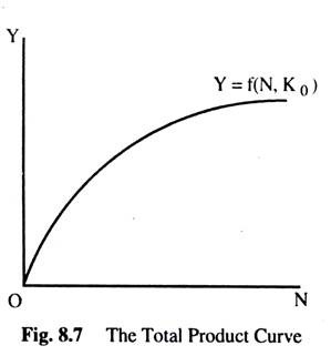
The aggregate production function gives us aggregate output as a function of the volume of employment, given the capital stock (K₀), which is constant in the short-run, and the level of output, which will increase as employment increases. The aggregate production function may be written as Y = f (N, K₀), where K₀ is a given capital stock and N is the volume of employment in the economy.

It is assumed that dY/dN > 0 and d²Y/dN² < 0 i.e. the marginal productivity f labour increases at a decreasing rate as more labour is employed. The total product curve is given in Fig. 8.7. The slope of the production function at any point gives the marginal productivity of labour and the shape of the curve reflects the assumption of the diminishing marginal productivity of labour.

The assumptions of perfect competition and profit maximisation will give us the demand curve for labour where the value of marginal product is equal to the money wage rate. If W is the money wage rate and P is the price level, the condition of profit maximisation can be written as w = p dY/dN.

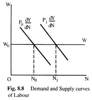
The demand curve for labour is determined from the aggregate production function. The labour demand curve is downward sloping as we have seen in the case of labour demand curve under classical system. For each price level we shall get one labour demand curve. For example, if the price level is P₀, the labour demand curve is p₀ dY/dN where dY/dN = MPP of labour.

Similarly, if the price level is P₁, the labour demand curve is P₁ dY/dN where P₀ < P₁. As the price level increases, labour demand curve shifts to the right as Fig. 8.8 shows.

The supply function of labour in the Keynesian system is totally different from that in the classical system. Keynes assumes that at the existing money wage rate W₀, there is a number of workers (N_f) who are willing to work, irrespective of price level. The money wage rate is assumed to remain fixed at the existing level, until full employment is reached.

When the full employment is achieved, money wage rate rises to induce an increase in the supply of labour. Keynes assumes that money illusion exists in the supply of labour function. When an individual is concerned not with the real value of money but only with the nominal value of money, the individual is said to be suffering from money illusion. This means that the supply of labour is a function of money wage rate.

There are several reasons for assuming that labourers suffer from money illusion. Firstly, Keynes thought that due to the growth of the trade unions, the workers will not accept a low money wage whatever the real wage rate may be. In other words, the money wage rate is rigid — at least in downward direction — and cannot fall below a certain level, though there is no such limit for real wage rate.

Secondly, workers have some fixed obligations in money terms. Even if money wages and prices tall, these obligations will not be reduced. Because of the existence of these obligations, the workers will not accept a cut in money wage rate even if all current prices are cut proportionately.

The Keynesian labour supply function may be written as:

W = W₀ + W (N) such that W(N) = 0 for N < N_f, and W'(N) > 0 for N > N_f.

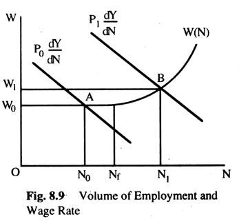
At a minimum money wage rate W₀, N_f workers are willing to work. This is called full employment level. This means that at the wage rate W₀ all workers are willing to work up to full employment. When the actual employment is less than or equal to the full employment level the money wage rate is constant. But if the volume of employment is greater than the full employ­ment level, the wage rate will increase as employment increases which is shown in Fig. 8.9.

In the vertical axis we plot the money wage rate and in the horizontal axis the volume of employment is measured. The money wage rate is constant at W₀ up to full employment level, N_f, thereafter it increases as employment increases. If N represents the supply of labour and W represents the money wage rate then the labour supply can be written as N = N (W).

In inverse form the Keynesian labour supply function is written as:

W = W (N).

Equilibrium in the labour market will be achieved where demand and supply of labour arc equal which is shown in Fig. 8.9. If the price level is assumed constant at P₁, the labour demand curve p₁ dY/dN cuts the supply curve at its upward rising point B where the equilibrium money wage rate is W₁ and employment is N₁. This is a full employment situation (as all willing to work at this wage rate (W₁) are employed).

However, if the labour demand function intersects the labour supply function at its horizontal part at point A, the equilibrium wage rate is W₀ and the equilibrium employment is N₀. At this situation, there is unemployment of N₀N_f. At the wage rate of W₀, ON_f workers are willing to work, but ON₀ workers are getting jobs.

Thus, N₀N_f workers are involuntarily unemployed. This is a condition of under­employment equilibrium which exists because of the shape of the labour supply function. This involuntary unemployment cannot be solved by reducing the money wage rate because it cannot fall any more.

The equilibrium position in the labour market will depend on the labour demand curve which depends on the price level. As price level changes, the labour demand curve also changes and hence the equilibrium level of un­employment. Unless we know the equilibrium price level, we cannot determine the equilibrium level of employment.

There is no guarantee that full employment will be automatically achieved in the labour market. If the labour demand curve intersects the labour supply at the latter’s horizontal part then full employment may not be achieved at all and involuntary unemployment may prevail. Thus, there is no automatic mechanism to achieve full employment in the labour market.

From the labour market, we shall get labour demand corresponding to price level. Given the supply of labour, the equilibrium level of employment can be determined. From the aggregate production function we know that as the level of employment increases so the level of output also increases. Thus, from the equilibrium in the labour market we can get different combinations of P and Y for which the demand for labour is equal to the supply of labour.

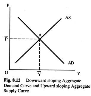
The aggregate supply curve will be upward rising. The aggregate supply (AS) curve shows the amount of output supplied at different prices. It is determined from the labour market which represents those combinations of P and Y for which the demand for labour is equal to the supply of labour. The labour market will always be in equilibrium at any point on the AS curve.

Mathematically, the AS curve can be derived as follows:

We have 3 equations for the labour market – Y = ф(N, K₀), W=P dY/dN and W = W₀ + W (N). Since we have 3 equations and 4 unknowns, we cannot solve for these 4 unknowns. So, we eliminate N and W and get a relation between Y and P which represents upward sloping AS curve for the economy.

From the equilibrium conditions in the commodity and money market, we can derive the aggregate demand curve. Suppose we derive LM curve for constant

Money supply M₀ and constant price level P₀ which represents those combinations of r and Y for which the demand for money is equal to the supply of money. We can also derive an IS curve which represents those combinations of r and Y for which investment equals saving.

The equilibrium level of income and interest rates are simultaneously determined by the intersection of IS and LM curves. Now, we assume that the supply of money remains constant at M₀ but the price level changes.

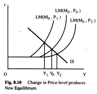
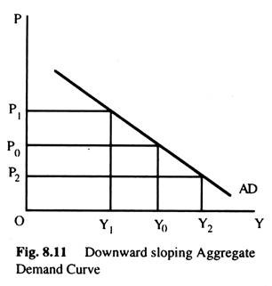
As a result, the LM curve will shift and we shall get a new equilibrium position and a new equilibrium level of income. This is shown in Fig. 8.10. For one price level we get one LM curve and one equilibrium level of income determined by the intersection of IS and LM curves. When the price level is P₀ and the money supply is M₀, we get one LM curve LM(M₀, P₀) and the equilibrium level of income Y₀ as in Fig. 8.10.

Now, suppose that the price level increases to P₁ and LM curve shifts to LM (M₀, P₁) and the equilibrium level of income to Y₁. If, however, the price level decreases to P₂, the equilibrium level of income increases to Y₂ and LM curve shifts to LM (P₂, M₀). By plotting the points (P₀, Y₀), (P₁, Y₁) and (P₂, Y₂) we get a downward sloping aggregate demand curve as shown in Fig 8 11.

From equilibrium conditions of the commodity and money market we get:

S(Y) = I(r) and M₀ = kYP + L₂(r).

In these two equations, we have three unknowns r, Y and P and, hence, we cannot solve for these unknowns. Thus, we eliminate r from these two equations and get a downward sloping relation between P and Y which gives us the aggregate demand curve for the economy.

Thus, we derive from the labour market different combinations of P and Y for which the labour market is in equilibrium. Again, from the money and commodity markets we get combinations of P and Y for which the money and commodity markets will be in equilibrium.

The first relation is known as the aggregate supply curve which is upward sloping and the second relation is known as the aggregate demand curve which is downward sloping. If we plot them together in a single diagram as in Fig. 8.12, the two curves intersect at point A which satisfies the equilibrium conditions in all three markets. More about AD and AS later on.

In the complete Keynesian model, economy is divided into four markets – the commodity market, the money market, the bond market and the labour market. It is the general equilibrium system where the equilibrium of the entire economy is considered. From the general equilibrium theory we know that if three out of four markets are in equilibrium the fourth market must also be in equilibrium. This is the Walras law.

According to Walrasian law, Keynes dropped the bond market from his analysis and considered equilibrium conditions in other three markets. If these three markets are in equilibrium then the bond market must also be in equilibrium. In each market there are three equations.

The complete Keynesian model will be described by the following equations.

The commodity market has the following three equations:

(1) S = S(Y) Saving function

(2) I = I(r) Investment function

(3) S = I Equilibrium condition.

In the money market, we have three equations:

(4) M_D = KPY + L(r) Money demand function

(5) M = M₀ Money supply function

(6) M_D = M₀ Equilibrium condition

The labour market has 3 equations:

(7) Y = f(N, K₀) Aggregate production function

(8) W = P dY/dN Labour demand function

(9) W = W₀ + W (N) Labour supply function

Thus, we have nine equations and nine variables – S, I, r, Y, L, M, P, N, W. The system can be solved and the unique equilibrium values of all the variables can be determined. Alternatively, equations (1) to (3) can be transformed into a single equation – (I’) S(Y) = I(r).

Equations (4) – (6) can be transformed into a single equation:

(2′) M₀ = KPY + L(r)

Equations (8) to (9) can be transformed into:

(3′) P dY/dN = W₀ + W (N)

Lastly, equation (7) can be written as:

(4′) Y = f (N, K₀).

Thus, we have four equations and four unknowns – Y, r, P and N. Note that equation (1’) and (2′) have three variables – Y, r and P. We can eliminate r and get a relationship between P and Y. This gives us the aggregate demand curve. Similarly, equations (3′) and (4′) give us the aggregate supply curve. At the intersection point of the aggregate demand and supply curves all four equations (1′) – (4′) are satisfied. Here the price level P acts as the linking variable between (f) – (2′) and (3′) – (4′).

Alternatively, we can write the system of equations with employment (N) as the linking variable. Let us rewrite the equations where we replace f (N,K₀) for Y. Equation (1′) can then be written as S{f (N, K₀)} = l(r)…………. (1″) Equation (2′) can be written as – M₀ = KPf (N, K₀) + L(r)………….. (2″) Equation (3′) is written as – Pf (N, K₀) = W₀ + W (N)……………… (3″).

Thus we have three equations and three unknowns – N. r and P. Now we consider first equations (1″) and (3″). Here we have three variables r, P and N. These can be solved for r and P in terms of N. By substituting the values of P and r in (2″), we get just one equation in one unknown – N and we can determine N from (2″). Once N is known r can be found from (1”) and P can also be found from (3″). In this way, the system can be solved. Thus, the Keynesian system is deterministic, but the full employment is not guaranteed.

Graphical Exposition of the Complete Keynesian Model:

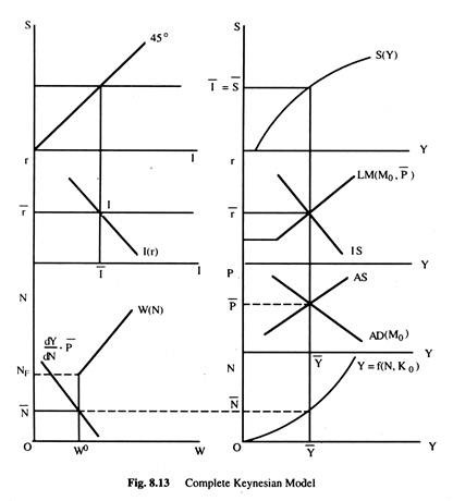
The complete Keynesian model can also be represented graphically by bringing together all the markets. We can identify from the diagram the equilibrium values of all the variables of the system. The Fig. 8.13 depicts the complete Keynesian model.

The figure shows the aggregate demand and aggregate supply (AS) curves. The aggregate demand curve is drawn on the assumption of a constant money supply M₀. The aggregate supply curve, AS, intersects the AD to produce equilibrium price level P̅ and the equilibrium output level Y̅, when the level of output is known, the corresponding level of employment N̅ can be obtained from the aggregate production function {r = f(N, K₀)}.

The labour demand and supply curves are drawn on the left hand side of the aggregate production function. The labour demand curve is drawn for the price level P̅. The labour demand curve intersects the labour supply curve to give us equilibrium employment N.

Since the labour demand curve intersects the labour supply curve at the latter’s horizontal part, there is involuntary unemployment of N_f – N̅. The equilibrium money wage rate is W₀. We have drawn the IS and LM curves above the AD and AS curves. The LM curve corresponds to the money supply M₀ and the equilibrium price level P. At the intersection of IS and LM curves the equilibrium rate of interest r is determined. From this diagram (Fig. 8.13), we can determine all important variables of the system.

Again, when Y is known, S can be determined from the saving function S(Y) which we have drawn above the IS-LM curves. When the equilibrium level of income is Y̅, the saving is S̅. The equality between saving and investment is shown through 45° line.

When the equilibrium rate of interest is known, the level of investment can be known from the diagram below the 45° line and to the left hand side of the IS-LM curves which give the equilibrium rate of interest. By extending the diagram, it is possible to show the transactions and the speculative demand for money separately which is avoided here.

In this way, all the equations of Keynesian model may be represented. The equilibrium system represented here is an underemployment equilibrium because there exists involuntary unemployment of N_f -N̅ which has been caused by wage rigidity. The full employment equilibrium may also be achieved if the labour demand curve intersects the supply curve at the latter’s upward rising part.

Effect of a Change in the Money Wage Rate in the Complete Keynesian System:

The labour supply function in the Keynesian model can be written as W = W₀+ W (N) where W₀ is the fixed money wage rate at which the labour supply function is horizontal. At this money wage rate N_f workers are willing to work. When the money wage rate, W₀, changes, its effects in the complete Keynesian model can be obtained by differentiating the equations of the Keynesian model with respect to W₀.

Let us examine whether a cut in the money wage rate can increase the level of employment and income or not. The effects of a cut in the money wage rate can be examined as follows.

A cut in money wage rate means a cut in real wage rate as well. As the real wage rate falls the level of employment and real income increases. As the money wage rate falls, the labour supply curve shifts in the downward direction and the aggregate supply curve also shifts in the same direction the price level falls which reduces the transactions demand for money. To maintain equilibrium in the money market the speculative demand for money must increase which means that the rate of interest must decrease.

The fall in price will increase the real wage rate. This will reduce income and employment. Thus, the initial increase in the level of employment will be offset by the price effect. When equilibrium is finally reached, the real income and employment will increase as the interest rate and the price level decrease.

Only exception to this general rule is when the liquidity preference function is perfectly interest-elastic, the interest rate does not fall (liquidity trap situation). A cut in the money wage rate will reduce the price level only but keeps the level of employment, income and interest rate unaffected.

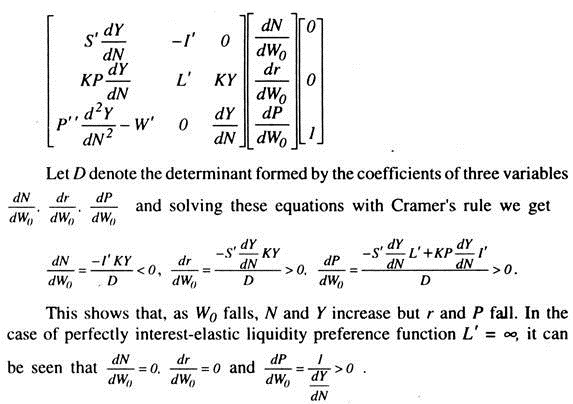
Mathematically, its effect can be derived as follows:

We consider three equations of the complete Keynesian system:

(1) S {f (N)}

(2) KPY + L(r) = M₀

(3) P dY/dN = W₀ + W (N)

Differentiating these three equations with respect to W₀ and rearranging we get the following:

It means that in the case of liquidity trap situation a fall in the money wage rate has no effect on the level of employment, income and the rate of interest. It leads to a fall in the price level only.

Effect of Change in Money Supply in the Complete Keynesian Model where the Price Level is Flexible:

In the Keynesian system, the equilibrium price level is determined by the intersection of aggregate demand and aggregate supply curves. When the aggregate demand curve is drawn, money supply is assumed to be constant. Thus, when the money supply increases the aggregate demand curve shifts to the right. The aggregate supply curve will not be affected by money supply as it does not enter into the determination of the aggregate supply curve.

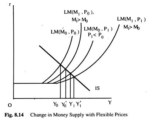
Let us now see how the AD curve will be affected when the money supply increases. In Fig. 8.14, we can see that, as the supply of money increases, the LM curve shifts to the right at each price level and, hence, the level of income will increase at each price level. When the price level is P₀ and the money supply is M₀, the equilibrium income is Y₀. When the supply of money increases to M₁, the equilibrium level of income will increase to Y₀, the price level remaining unchanged.

Similarly, when the price level is P₁ and money supply is M₀, the equilibrium income is Y₁. Now if the money

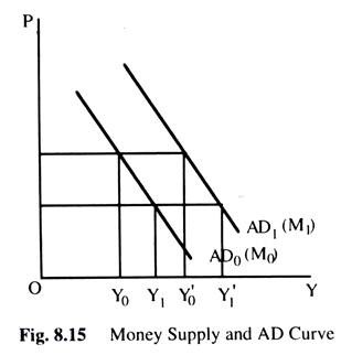
supply increases to M₁, the equilibrium level of income increases to Y₁. Thus, we see that, as the money supply increases, at each price level a higher level of income will be required, to have equilibrium in commodity and money markets. This means that the AD curve will shift to the right as in Fig. 8.15.

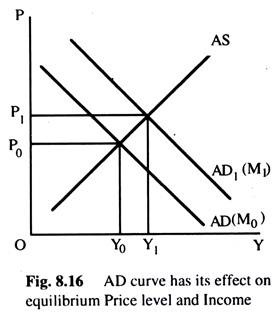
When the aggregate demand curve shifts to the right, the equilibrium price level increases from P₀ to P₁ and the equilibrium income also increases from Y₀ to Y as in Fig. 8.16.

As the level of income increases, the rate of interest falls. Moreover, the value of employment will increase as total output increases. The price level increases and the labour demand curve shifts in the upward direction. If the labour demand curve intersects the labour supply curve at the latter’s rising part then the money wage rate will increase.

Otherwise, it will remain unchanged. Since employment can increase if the real wage rate falls, it must fall when the money supply increases. This means that the price level must increase rapidly than the money wage rate if the real wage rate is to fall.

Effect of Change in Autonomous Investment in the Keynesian Model:

Here we will consider the effect of change in autonomous investment on the equilibrium values of the variables in the Keynesian model. Suppose autonomous investment increases which will shift the investment function in the upward direction.

So the AD curve shifts in the upward direction as well. However, the aggregate supply curve remaining the same when the AD curve shifts in the upward direction, the equilibrium price and income increase. As real income increases, the level of employment also increases.

Furthermore, when the price level increases, the demand for transaction balances increases and the money market equilibrium requires that the speculative balances should decrease. This means that the interest rate should increase which will reduce induced investment and also the aggregate demand. This process continues until a new equilibrium is established.

Thus, the effects of an increase in autonomous investment can be summarised as follows:

a higher level of employment and income, a higher interest rate and price level and a lower real wage rate.

There are two limiting cases in which this result will not follow. Firstly, if the liquidity preference function is perfectly elastic and, secondly, it the speculative demand for money is zero.

Limitation of the Keynesian Theory:

After the World War II, Keynesian demand-management policies were used by the governments of most Western developed economies in an attempt to keep down unemployment which was the main economic problem. Generally, these policies were successful in preventing unemployment like that experienced in the 1930s, but, unfortunately, they tended to give rise to the phenomenon known as stop-go.

That is, in a period of high unemployment, the government used to expand aggregate demand; which would reduce unemployment but at the same time give rise to inflationary situation so that the government eventually would have to reduce aggregate demand. Thus, all go periods used to be followed by stop period and it became difficult to achieve long-run economic growth. This is mainly because the Keynesian model is a short-term one and in the short-run the management of the economy may become very erratic.

A second limitation of the model as we have pointed out in this chapter is that it fails to take into account the problem of inflation. Indeed, the basic model assumes that prices and wages are fixed and the only time they were allowed to rise is after the attainment of full employment. Experience in 1970s has shown us that high rates of inflation can co-exist with high rates of unemployment and no explanation is provided in the Keynesian theory. Furthermore, the coincidence of inflation and unemployment makes the Keynesian policy recommendations questionable.

A further criticism that has been levelled against the Keynesian model is that it tends to understate the influence of money on the real variables in the economy. We have already seen that a change in the money supply in this model affects national income through its effect on the rate of interest; it is because of this that Keynesians put more faith in fiscal rather than monetary policy.

Monetarists have been mainly concerned with these three criticisms of the Keynesian theory.

They also make the following points:

(a) that short- term demand may do more harm than good;

(b) that there is a close relationship between changes in the money supply and changes in money national income in the long-run.;

(c) that without government interference the economy will tend towards natural rate of unemployment.

Some Special Criticisms of the Keynesian Model:

There are two general criticism of the Keynesian model. Firstly, the Keynesian model is “too aggregative”. Secondly, this model is too static. It means that the model does not consider the short-run dynamics of income change and that it is unsuitable to the analysis of long-term economic growth. The model is a short run model in that it assumes a given capital stock. Keynes was interested in the short run as he said, “in the long run we are all dead”.

The Keynesian model can be dynamised at least in two directions. Firstly, it is possible to introduce time lags in different functions and analysis of the time path to achieve different equilibrium values. Secondly, it may be possible to consider the effect of an increase in the capital stock on the equilibrium values of different variables. The model is “too static” for the analysis of either the problems of economic growth or the business cycle.

Apart from these general criticisms, we can advance some criticisms devoted to the specific parts of the Keynesian model.

Firstly, the Keynesian liquidity preference function has been criticised mainly on the ground that he considered only two assets — money and bonds. This is an over-simplification. In the real world, there are different types of monetary and non-monetary assets. All these are considered in the modern portfolio approach to the demand for money. Keynes’ division of the demand for money into three parts — transaction demand, precautionary demand and speculative demand — has also been criticised. It has been argued that it is difficult to separate between units of money held for speculative and transaction purposes. The same unit of money may be used for either purpose.

Secondly, the Keynesian investment theory has been criticised and new theories have been offered as an alternative to the Keynesian theory which have been discussed later in this book.

Thirdly, the Keynesian consumption function has been criticised and several alternative hypothesis has been developed which we consider later on.

Fourthly, the hypothesis that firms maximise profits has been criticised. Recent developments of the theory of firms show that the objective of the modern firms is not only the maximisation of profits. There are alternative objectives such as sales revenue maximisation and managerial utility maximisation and so on.

Fifthly, the theory of money wage determination in the model is inadequate.

Sixthly, Keynes did not consider the “Real balance effect” or the Pigou effect of the flexibility of the price level in the face of unemployment.

Lastly, unemployment is today’s problem. But the greatest problems in the modern world are associated with inflation and economic growth. The Keynesian analysis is incapable of dealing with these twin problems. Keynes was mainly concerned with unemployment in the short run. He did not consider the problem of economic growth or inflation. He was mainly concerned with the problem of depression. However, attempts have been made in recent years to extend the Keynesian analysis to the problems of inflation and economic growth.