Role of Inventory Changes in SKM | Simple Keynesian Model

Role of Inventory Changes in SKM!

In SKM the equilibrium condition of Y, in terms of leakage injection approach, is

I̅ + Δinv + G = S + T …(15)

where Δinv represents unexpected, or involuntary, inventory changes. This equation is true, by definition, all the time. But income is at its equilibrium level — that is, sales are going as expected — only when Δinv is zero, and

I̅ + G = S + T = S(Y- T(Y)) + T(Y) … (16)

Here we introduce the dependence of saving and tax revenues on Y. Equation (16) is an equilibrium condition for income Y.

When income is at the level where saving plus tax revenue (as functions of income) equal planned investment plus government spending, then unex­pected Δ inv equals zero, sales expectations are being realised, and there is no tendency for income and output to change. If income is higher than that level which satisfies equation (16), (S + T) will exceed planned (I̅ + G), sales will be low, and Δinv will be positive.

The identity (5) will still hold with Δinv = (S + T) – (I̅ + G), but income will not be at its equilibrium level because sellers will be cutting back orders to reduce unwanted inventory stocks, and production and income will be falling. This will continue until income falls enough to bring (S + T) down to (I + G) and reduce Δ inv to zero, bringing sales expectations and realisations back in line with each other.

Thus, at an initial level of income Y₀, (S + T) exceeds (I̅ + G), Δinv is positive. If this is the case, the economy is not in equilibrium because final sales are less than what producers and sellers expected. Therefore, producers will reduce their expectations and begin to reduce production.

As they do that, income will fall. Conversely, if (S + T) is less than (I̅ + G), Δinv must be negative, producers will expand output to meet the unexpected in­crease in demand, and income will rise.

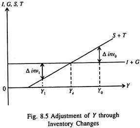
The determination of the equilibrium level of income is shown graphically in Fig. 8.5. In Fig. 8.5, S + T has positive slope because here we assume that both S and T are increasing functions of Y. We also as­sume that I̅ and G are fixed independently of the level of Y, so that the I̅ + G line is horizontal.

The point at which is S + T = I̅ + G, that is, where the two lines cross, determines the equilibrium level of income Y_e that satisfies equilibrium condition (16).

We can further see that this equilibrium is a stable one. In other words, if external forces cause the system to move away from the equilibrium point, it will tend to settle back to equilibrium at Y_e. At a level of income Y₀ in Fig. 8.5 to the right of Y_e, saving plus tax revenue is greater than planned I̅ + G.

This means that people are buying less than sellers expected at that level of income causing an unexpected inventory accumulation of amount Δ inv_Q. The inventory accumulation is just enough to maintain the saving-investment balance in the national income accounts, since, at Y₀,

I̅ + G + Δinv₀ = S(Y₀ – T(Y₀)) + T(Y₀.)

But since Δ inv₀ is positive, producers will cut back on production, causing income to fall toward Y_e. Conversely, to the left of Y_e, where income is at Y₁, saving plus tax revenue is less than I̅ + G. This means that people are buying more than sellers anticipated, causing an unexpected reduction of inventories of amount Δ inv₁.

Producers will then expand production to satisfy this greater demand, causing income to increase toward Y_e. Thus, the equilibrium level of income, Y_e, is stable. When actual income is below equilibrium Y_e, Δ inv is negative and production and income are rising. When actual income exceeds Y_e, Δ inv is positive and income is falling. Only at Y_e is there no tendency for income to change.

This explanation of the equilibrium level of income contains one important oversimpli­fication. At Y₀ unexpected inventories accumulated, causing producers to reduce their production until there was no further unexpected inventory accumulation at Y_e, where Δ inv is zero.

However, although no new unwanted inventories are accumulated at Y_e, producers and sellers are still faced with that unwanted stock of inventories that accumulated before they made their adjustments.

In order to work-off that stock, they may cut intended inventory accumulation slightly, shifting the I̅ + G line of Fig. 8.5 down a bit as excess inventories are reduced. Eventually, though, the desired level of inventory accumulation included in I̅ will return to its original level, and equilibrium income will be restored at Y_e.

A simple example will make the SKM quite clear to us.

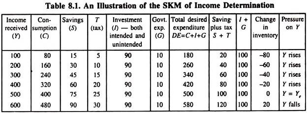
Table 8.1 gives a simple illustration of the Simple Keynesian Model of Income Deter­mination (figures in Rs. crores).

Here we assume that MPC is 4/5. We also assume that I = I̅ = 90 and G = G̅ = 10 at all levels of income. Thus when Y is 100, C + I + G is 180. So there is unintended inventory shortfall of 80. This will cause output to rise in order to meet the excess demand pressure. When output increases to 500, there is no unintended shortfall of inventories.

Current output is just sufficient to meet current demand. Actual (realised) investment is equal to desired investment (which also includes desired inventory investment) and undesired inventory investment is zero.

If producers overreact to the excess demand pressure and produce an output of 600, there will be the problem of excess supply (surplus). So there is undesired accumulation of inventory of 20. This will cause output to fall to the equilibrium level (500).

Thus only when Y = C + I + G, national income attains its equilibrium value. At this level of income S + T = I + G = 100. Since Y=a + bY, S = Y – C = Y – a – bY = – a + (1 – b)Y. So both the conditions of national income equilibrium are satisfied in the Keynesian model.