Monetary and Fiscal Policy: Effects and Changes (With Diagram)

Let us make an in-depth study of the Monetary and Fiscal Policy. After reading this article you will learn about: 1. Effects of an Increase in Expenditure and Taxes 2. Monetary Policy Changes and Shift of the LM Curve 3. The Relative Effectiveness of Monetary and Fiscal Policies.

Effects of an Increase in Expenditure and Taxes:

(i) Effect of an Increase in Government Expenditure:

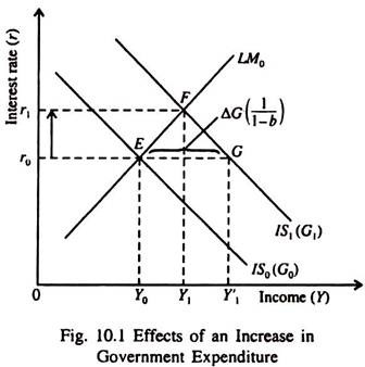
An increase in government expenditure shifts the IS curve to the right from IS₀ to IS₁, as shown in Fig. 10.1. As a result income rises from Y₀ to Y₁.

This increases the transactions demand for money and reduces the demand for bonds and causes the price of bonds to fall or the interest rate to rise (even if the LM curve does not shift).\

Since money supply remains fixed, total money demand cannot increase.

The attempt to hold more money will raise the rate of interest, reduce the speculative demand for money and cause people to economise on the amount of trans­action balances held for any level of income. At new equilibrium, the rate of interest must rise sufficiently so that net money demand remains unchanged even at a higher level of income.

The IS-LM curve model includes a money market, which does not exist in the SKM. So when G increases, r must rise to maintain equilibrium in the money market. In Fig. 10.1 we see that Y rises by less than the amount by which G increases.

The reason is that the rise in interest rate from r₀ to r₁ chokes off investment demand and thus aggregate demand and partly offsets the increase in income that would occur due to a rise in G in the absence of a rise in r.

Thus the increase in income in the IS-LM curve model is less than that in the SKM, here the SKM overstated the effect of an increase in G by assuming investment as completely autonomous and neglecting the necessary increase in r and consequent decline in I that accompany an increase in G.

(ii) Effect of an Increase in Taxes:

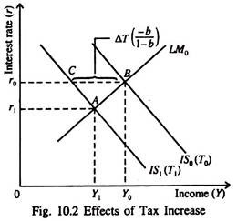
An increase in taxes from T₀ to T₁ shifts the IS curve to the left for IS₀ (T₀) to IS, (T₁). Since taxes are a leakage from the circular flow of income, Y falls from Y₀ to Y₁ rates falls from r₀ to r, market equilibrium.

In this case Y falls by less than the horizontal distance FG by which the IS curve shift. Here FG = ΔT[- b / 1-b] the tax multiplier from the SKM times the change in tax total. Thus effects of fiscal policy multipliers are less than those in the SKM. In this case the fall in r will cause investment to rise.

This will partly offset fall in consumption caused by the tax increase (AT). The SKM assumed investment to be autonomous and hence fixed at all levels of income Y, and so neglected this offset, and hence overstated the effects of the tax increase.

(iii) Effect of an Autonomous Fall in Investment:

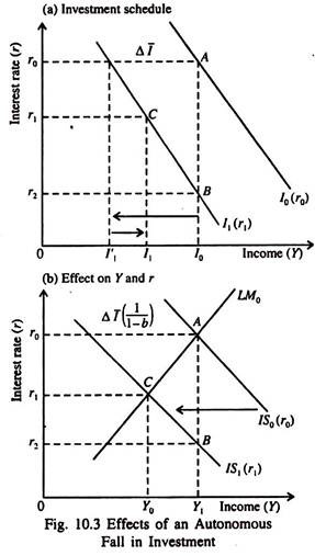
Fig. 10.3 shows the effect of an autono­mous fall in investment. In part (a) the invest­ment demand curve shifts to the left. At the original rate of interest r₀, the level of invest­ment falls from I₀ to I’₁. The shift of the investment function causes the IS curve in part (b) to shift to the left from IS₀ to IS₁.

As a result equilibrium income falls from Y₀ to Y₁, and equilibrium rate of interest also falls from r₀ to r₁. Due to a fall r, investment increases to some extent from I’₁, to I₁, in part (a). If the interest rate falls to r₂, the investment returns to the original level I₀.

This will happen if the LM curve is vertical. If the LM curve is vertical a shift of the IS curve to the left from IS₁ to IS₁ will leave Y unchanged but cause r to fall from r₀ to r₂. Thus for income to remain unchanged with an autonomous decline in investment, the rate of interest would have to fall to r₂. However, if the interest rate falls to r₁, the autonomous fall in investment is partly offset.

Monetary Policy Changes and Shift of the LM Curve:

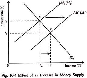
If money supply increases from M₀ to M₁ the LM curve shifts to the right from LM₀ (M₀) to LM₁, (M₁) as shown in Fig. 10.4. As a result the equilibrium rate of interest falls from r₀ to r₁ and income rises from Y₀ to Y₁. Due to a rightward shift of the LM curve, there is excess supply of money which causes r to fall.

As r falls, investment demand increases and this causes Y to rise, with a further income-induced increase in consumption spending. A new equilib­rium is attained at point F when the fall in r and the rise in Y jointly increase the demand for money exactly by the amount by which money supply has increased initially. This equilibrium occurs at point F where the new LM curve intersects the IS curve.

An increase in demand for money for given levels of income and the interest rate will shift the LM curve to the left. As people shift their portfolio of wealth and increase their money holding (or reduce their bond holding), the rate of interest will rise.

This will reduce investment and equilibrium income. Such a shift implies that more money is demanded at a given level of income and interest rate. This has the same effect as a fall in money supply.

Fiscal-Cum-Accommodating Monetary Policy:

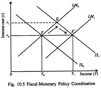
By making appropriate use of monetary and fiscal measures it is possible to achieve the best of both the worlds — an increase in Y without permitting r to rise. The effect of such a policy mix is illustrated in Fig. 10.5.

Fig. 10.5 shows that a tax cut or an increase in government expenditure shifts the IS curve to the right from IS₀ to IS₁. As a result equilibrium income will rise from Y₀ to Y₁ and equilibrium r from r₀ to r₁.

However, if expansionary fiscal policy is accompanied by an expansionary monetary policy in the form of an increase in money supply from M₀ to M₁, the LM curve will also shift to the right from LM₀ (M₀) to LM₁ (M₁).

This will offset the rise in r that would occur in the absence of monetary policy change. In this case we have illustrated the Keynesian presumption of fiscal policy actions such as income tax cuts to expand the economy supported by an accommodating mon­etary policy — an accompanying in­crease in the money supply that will prevent r from rising and preventing crowding out of investment.

In Fig. 10.5 at the same time the IS curve is shifted to the right by a tax cut, the supply (stock) of money is increased sufficiently so that the LM curve shifts far enough to the right to prevent a rise in r.

Table 10.1 summarises the effects of changes in fiscal and monetary policy variables.

If money supply (M) rises, Y rises, but r falls. If government expenditure (G) increases, Y and r both rise. If tax total (T) rises, Y and r both fall.

The Relative Effectiveness of Monetary and Fiscal Policies:

Both fiscal and monetary policy instruments can affect the level of income. We may now examine the relative effectiveness of the two types of policies. By effectiveness we mean the magnitude of the effect on equilibrium income Y of a given change in the policy variable such as G, T, or M.

It may be noted at the outset that the effectiveness of each type of policy – fiscal or monetary — depends on the slopes of the IS and LM curves, which in turn depend on certain behavioural parameters of the IS-LM curve model.

i. The Slope of the IS Curve and the Effectiveness of Fiscal Policy:

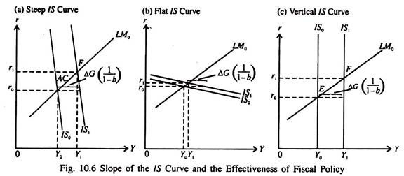
In each part of Fig. 10.6, an increase in G shifts the IS curve to the right from IS₀ to IS₁. In part (a), where the IS curve is steep, this expansionary fiscal policy action (in the form of an increase in G or a cut in T or both) results in a relatively large increase in Y.

The same fiscal policy action is much less effective (Δ Y is much smaller) in part (b), where the IS curve is relatively flat. Fiscal policy is most effective in part (c), where the IS curve is vertical.

ii. The Slope of the LM Curve and the Effectiveness of Fiscal Policy:

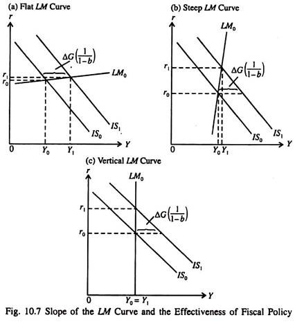
In each part of Fig. 10.7, an increase in G shifts the IS curve to the right from IS₀ to IS₁. Fiscal policy is most effective in part (a), where the LM curve is relatively flat; less effective in part (b), where the LM curve is steeper; and completely ineffective in part (c), where the LM curve is vertical.

iii. The Slope of the IS Curve and the Effectiveness of Monetary Policy:

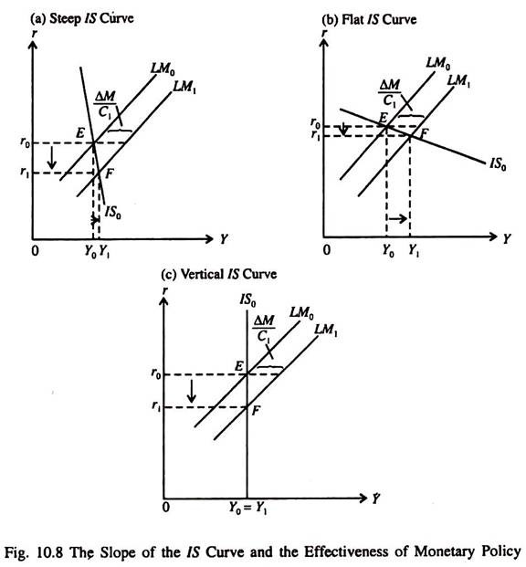
An increase in the money supply shifts the LM curve to the right from LM₀ to LM₁ in Fig 10.8. This expansionary monetary policy has only a small effect on Y in part (a), where the IS curve is steep. It has a much stronger effect on Y in part (b), where the IS curve is relatively flat.

In part (c), where the IS curve is vertical, the income in money supply has neutral effect on equilibrium income.

iv. The Slope of the LM Curve and Effectiveness of Monetary Policy:

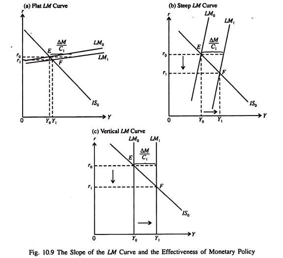
In each part of Fig. 10.9, an increase in money supply shifts the LM curve to the right from LM₀ to LM₁. Monetary policy is least effective in part (a) where the LM curve is relatively flat; more effective in part (b), where the LM curve is steeper; and most effective in part (c), where the LM curve is vertical.

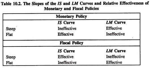
Table 10.2 summarises the points concerning the relative effectiveness of fiscal and monetary policy changes in the context of the slopes of the IS and LM curves.

Complete Ineffectiveness of Monetary Policy in a Liquidity Trap Situation:

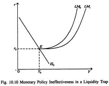
At the low levels of the interest rate that would prevail in the liquidity trap conditions, Keynesian model would expect the economy to be on the horizontal range of the LM curve, as shown in Fig. 10.10. Monetary policy would lose its effectiveness in this situation completely because monetary expansion can no longer reduce r and stimulate I.