The Keynesian Macroeconomic System (With Diagram)

Let us learn about the Keynesian Macroeconomic System. After reading this article you will learn about: 1. Introduction to The Keynesian Macroeconomic System 2. Goods Market Equilibrium: The IS Curve 3. Money Market Equilibrium: The LM Curve 4. Combining Goods Market and Money Market: General Equilibrium 5. Shifts of the IS and LM Curves: Effects of Fiscal and Monetary Policy Change and Other Details.

Introduction to The Keynesian Macroeconomic System:

We have said earlier that equilibrium level of income is determined by aggregate demand which is composed of consumption and investment expenditures (assuming a private sector economy without any trade).

Keynesian system involves six functional relations, viz. consumption function (or the saving function), the investment function, the demand function for money, aggregate production function, the demand function for labour, and the supply function of labour. Keynes’ saving function, money demand function, and labour supply function are really different from that of the classical system.

The primary determinant of Keynes’ saving function is income rather than the classical rate of interest.

That is,

S = f (Y) …(10.24)

Keynes added the speculative demand for money, L(r), to classical transaction demand for money, kPY.

Thus, Keynes’ money demand function is written as

M = kPY + L(r) …(10.25)

where speculative demand for money depends on the rate of interest, r.

Keynes’ labour supply function is assumed to depend on money wages which are institutionally rigid in the downward direction.

Thus, labour supply function is

S_L = f (W) …(10.26)

Where, W is the money wage.

However, the aggregate production function, investment function, and labour demand function of Keynes do not differ from the classical forms.

Keynesian income determination theory can explain macroeconomic problems once we incorporate money market in our analysis. It is the rate of interest, determined by the demand for money and the supply of money that integrates goods market and money market. Rate of interest not only influences investment but also (speculative) demand for money.

Thus, a synthesis of income and monetary analysis is brought about by the interest rate. Equilibrium national income is determined in the goods market when saving, equals investment. Monetary equilibrium is attained in the money market when demand for and supply of money are equal to each other.

By establishing equilibrium in the goods market and money market, equilibrium level of national income and the rate of interest are simultaneously determined.

To establish ‘general equilibrium’, we use the Hicks- Hansen tool, most popularly known as the IS- LM tool. The IS-LM analysis, a neo-Keynesian analysis, explains Keynesian macroeconomic system that takes into account goods market and money market simultaneously.

Goods Market Equilibrium: The IS Curve:

Keynesian theory of aggregate demand is inadequate to explain macroeconomic system when the money market is introduced. So, we need to establish a link between the money market and the goods market through the rate of interest. Now, we treat interest rate as a variable whose equilibrium value is determined simultaneously with that of the level of income.

In the goods market, we have:

(a) The saving function

(b) The investment function

(c) An equilibrium condition.

These are expressed as:

S = f (Y) …(10.24)

I =f (r) …(10.14)

and S = I …(10.27)

To develop the IS curve our task is to find combinations of interest rate, r, and the level of income, Y, that equate investment with saving. We cannot solve equation (10.27) for Y to determine equilibrium Y, unless we know Y. If ‘r’ is unknown, we cannot find out the volume of investment expenditure. At a given ‘r’, one can determine the volume of investment expenditure.

Once we determine investment expenditure, we are able to find out the equality between investment and saving. Consequently, equilibrium national income is determined in the goods market. In fact, there are a series of combinations of r and Y that ensure equality between saving and investment.

Once these combinations are plotted on the r – Y plane, we get a curve which Hicks-Hansen called the IS curve. The IS curve shows alternative combinations of national income (Y) and the rate of interest (r) which equilibrate the commodity market. Mathematically, the IS curve is simply the solution of equation (10.27) for r in terms of Y.

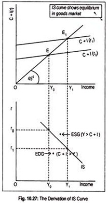
Fig. 10.27 illustrates the construction of the IS curve. In the upper panel of the figure, we have drawn the aggregate expenditure (C + I) schedule. National income is determined at that point where the aggregate demand line cuts the 45° line. We start with the given rate of interest.

Suppose, the initial rate of interest is r₀. At this rate of interest, aggregate demand schedule, C + I (r₀), cuts the 45° line at E. The corresponding level of income is Y_Q. As investment is inversely related to the interest rate, decrease in the interest rate from r₀ to r, causes investment to rise. Consequently, aggregate demand line shifts up to C + I (r₁).

The new aggregate expenditure schedule cuts the 45° line at E₁ and the corresponding level of national income rises to Y_r Thus, for the interest rate r₀, a point of product market equilibrium will be Y₀.

This r₀ – Y₀ combination is one point on the IS curve, shown in the lower panel of Fig. 10.27. Similarly, r₁ interest rate produces Y₁ equilibrium income. So, r₁ — Y₁ combination is another point on the IS curve. By joining these points we get a curve known as the IS curve.

Thus, the IS curve is the locus of all equilibrium combinations of r and Y that bring product market in equilibrium.

Any point off the IS curve shows disequilibrium in the goods market. To the right of the IS curve, there occurs excess supply of goods (ESG) when aggregate output exceeds aggregate demand, i.e., Y > C + I. To the left of the IS curve there arises excess demand for goods (EDG) when aggregate demand exceeds aggregate output, i.e., C + I > Y.

Thus the effect of an increase in r is:

r ↑→ I↓→ AD ↓→Y↓, and the effect of a fall in r is:

r ↓→ I ↑→ AD↑→ Y↑

The IS curve slopes downwards to the right. Or it has a negative slope.

Its slope depends on the saving function and investment function. The IS curve will be relatively steep (flat) if investment is less (more) sensitive to interest rate changes. The IS curve will be vertical if investment is absolutely interest-inelastic. An autonomous increase in investment expenditure or government expenditure will shift the IS curve to the right.

(a) Alternative Method of Deriving the IS Curve:

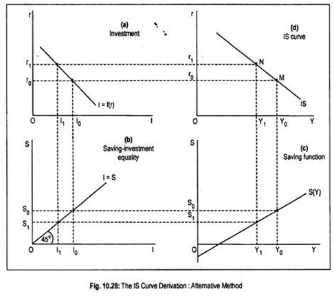
The derivation of IS curve can be made in terms of the four-part diagram (Fig. 10.28). In part (a), we have drawn investment function that shows the inverse relationship between investment and the rate of interest. Part (c) plots the saving function that represents direct relationship between income and saving. Part (b) is simply a 45° identity line, and part (d) plots the IS curve.

Suppose the rate of interest is r₀. At this rate of interest, investment must be I₀ and, thus, the volume of saving must be S₀, necessary for equilibrium. This volume of saving implies an equilibrium income of Y₀ necessary for equilibrium. This establishes one point on part (d), say point M. If the rate of interest rises to r_1; investment declines to I₁. This results in a decline in national income to Y₁.

With this level of income the volume of saving becomes S₁. This establishes another point on part (d), say point N. The procedure may be repeated for each level of income (interest) to obtain corresponding values of interest rate (income value) that ensure equality between saving and investment. By joining all these equilibrium points we get an IS curve drawn in part (d).

Thus, the IS curve shows various combinations of income and interest rate that brings the commodity market in equilibrium. The IS curve is negatively sloped. Its slope depends on the nature of saving and investment functions.

The IS curve may shift if there is a change in autonomous private investment and government expenditure.

Properties of the IS Curve: A Summary:

i. The IS curve is the equilibrium combinations of income and interest rate such that the product market or goods market is in equilibrium.

ii. The IS curve slopes downward to the right because an increase in interest rate causes investment expenditure to decline, therefore, reduces aggregate demand and, hence, equilibrium national income.

iii. Its slope depends on the saving and investment functions. The IS curve will be relatively steep (flat) if investment is less (more) sensitive to interest rate changes.

iv. This IS curve will shift by an autonomous change in investment spending or government spending.

v. Any point on the IS curve shows that there is neither excess supply nor excess demand for goods. Any point off the IS curve shows either excess supply of goods (ESG) or excess demand for goods (EDG).

Money Market Equilibrium: The LM Curve:

Equilibrium in the money market occurs at that point where money demand equals money supply. In the Keynesian system, money demand for transaction purposes depends on the level of income and money demand tor speculative purposes depends on the rate of interest.

Thus, the money demand function, denoted by M_d, can be expressed as:

M_d = f(Y, r) …(10.28)

Supply of money (M) is institutionally given. Given M, corresponding to each level of income there is a rate of interest which produces equilibrium in the money market. Money market equilibrium occurs when

M = M_d …(10.30)

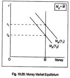
The LM curve shows different combina­tions of r and Y that equilibrate money market. In Fig. 10.29 we have drawn two money demand schedules, corresponding to two different levels of income. At Y₀ income, money demand schedule is given by M_d (Y₀). As income increases from Y₀ to Y₁, the money demand curve shifts to the right. The vertical line M shows fixed money supply.

We find equilibrium in the money market when money demand schedule intersects money supply schedule.

We start with a given income, Y₀. At Y₀ level of income, money demand schedule is M_d (Y₀). The rate of interest is r₀. As income rises to Y₁, money demand schedule shifts to M_d(Y₁) and the rate of interest rises to r₁. Thus, we find a direct relation between money demand and interest rate at different levels of income.

The effect of an increase in Y is:

Y ↑→ Md↑→ r↑ and the effect of a fall in Y is:

Y↓→M_d ↓→r ↓.

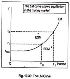
The interest-income combination at which equilibrium occurs, (r₀ – Y₀) and (r₁ – Y₁), are points along the LM curve. These points are plotted in Fig. 10.30. Thus, the LM curve is the locus of all combinations of r and Y that bring money market in equilibrium.

This LM curve slopes upward to the right because as interest rate rises equilibrium income rises. The slope of the LM curve depends on the interest elasticity of money demand. If interest elasticity of money demand is interest-inelastic the LM curve will be steep and if money demand is assumed to be highly interest-elastic, the LM curve will be flatter.

In an extreme case, if money demand is assumed to be perfectly interest-elastic (it happens at the floor rate of interest or the so-called liquidity trap region) the LM curve becomes perfectly elastic at this region. In Fig. 10.30 the LM curve is drawn parallel to the horizontal axis at the minimum rate of interest, r_min. The LM curve becomes positively sloped above the r_min range.

Any point off the LM curve shows disequilibrium in the money market. Just to the right of the LM curve there arises excess demand for money (EDM) and to the left of the LM curve excess supply of money (ESM) arises.

(a) Alternative Method of Deriving the LM Curve:

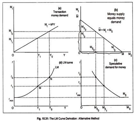
A four-part diagram may be used to derive the LM curve. Fig. 10.29(a) shows a proportional relationship between money income and transaction demand for money (M_t = kPY). Part (c) represents speculative demand for money [M_S = fir)]. The schedule in (b) is an identity line that mechanically divides money supply into transaction and speculative elements. Part (d) represents the LM curve.

Suppose, rate of interest, r₀, is known. Given r₀, the volume of speculative demand for money is M_S0. Given the total money supply (M), money not used for speculative purposes must be held for meeting transaction demand for money. Thus, the transaction demand must be M_t0. To ensure this transaction demand for money there must be a level of income Y₀.

Thus, we see in part (d), for interest rate r₀, the only possible money market equilibrium value for income is Y₀. If the rate of interest declines to r₀, the equilibrium level of income will be Y₁. The procedure can be repeated such that equilibrium combinations of r and Y emerge to ensure equality in the money market.

By joining all these combinations (M and N), we get the LM curve drawn in part (d). Note that at a floor interest rate, r_min, money demand becomes infinitely elastic. This makes speculative demand for money (shown in part c) to become horizontal at the minimum rate of interest. Because of this liquidity trap, the LM curve also becomes perfectly elastic. Anyway, the LM curve slopes upward from left to right.

Properties of the LM Curve: A Summary:

i. The LM curve consists of equilibrium combinations of income and interest rate for the money market.

ii. The LM curve slopes upward to the right.

iii. The slope of the LM curve depends on the interest elasticity of money demand. The LM curve will be (flat) steep if the interest-elasticity of money demand is relatively (low) high.

iv. The LM curve shifts due to changes in money supply and money demand.

v. All points on the LM curve show money market equilibrium such that there is neither excess demand for money (EDM) nor excess supply of money (ESM). Any point off the LM curve exhibits either EDM or ESM.

Combining Goods Market and Money Market: General Equilibrium:

Goods market and money market do not operate independently—one influences the other. Thus, combining these two markets, we can determine the values of Y and r that are consistent with equilibrium in these two markets.

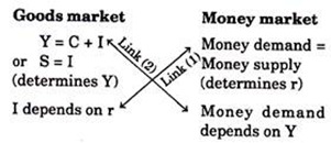
The interrelationships or the links between these two markets are:

There is a link between investment and interest rate determined in both the goods market and money market. Investment here is assumed to be determined by the interest in a negative fashion. We have amply demonstrated here that the interest rate is determined in the money market. Thus, money market influences goods market.

Another link can be traced between output/income and demand for money. We have seen that aggregate output determined in the goods market influences demand for money. An increase in income (keeping interest rate constant) causes an increase in money demand.

These two links can be shown in the following form:

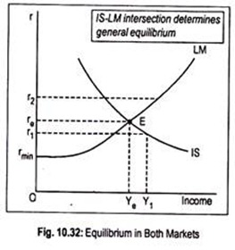
Fig. 10.32 shows the general equilibrium in terms of IS and LM curves. Here, when both the curves are plotted on the same axes, the equilibrium level of income, Y_e, and the equilibrium interest rate, r_e, are determined simultaneously.

This is known as the synthesis of monetary analysis and income analysis or macroeconomic general equilibrium. Point E is the (only) point of general equilibrium for both the markets. Point E is a stable equilibrium point.

To demonstrate stability, let us consider r₁ – Y₁ combination. Since this combination is on the IS curve, the product market is in equilibrium while money market is not. At this combination, there is an excess demand for money (EDM). To meet this excess demand, people will go on selling bonds.

This will depress bond prices and raise interest. As interest rate increases, there are repercussions in the product market. Now, following an increase in interest rate, investment declines and, as a consequence, income declines. So, interest rate and national income will go on changing until point E is reached, if the equilibrium is to be a stable one. This occurs only at r_e and Y_e.

Similarly, any r – Y combination above r_e will exhibit equilibrium in the money market, but disequilibrium in the product market. Now, product market will experience a deficiency in aggregate demand. This causes income to decline. As income declines, there are repercussions in the money market. Now, demand for money will decline as income declines. So, rate of interest must decline. If equilibrium is stable, r and Y tend to change until point E is reached. Thus, E is a stable equilibrium point.

One thing should be borne in mind—to have stability in equilibrium, the slope of the IS curve should be less than that of the LM curve.

Shifts of the IS and LM Curves: Effects of Fiscal and Monetary Policy Change:

It may be noted that the fiscal policy change (a change in taxes or government expendi­tures) will shift the IS curve, and monetary policy change will shift the LM curve.

(a) Monetary Policy:

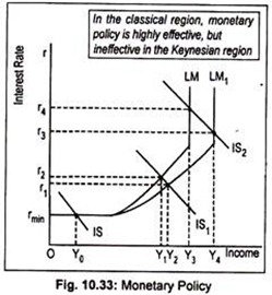
Monetary policy attempts to stabilize the aggregate demand in the economy by regulating the money supply. An expansionary monetary policy is needed to stimulate the economy. This makes the LM curve to shift to the rightward direction. Note that, in Fig. 10.33, we have drawn negative sloping IS curve and positive sloping LM curve.

The LM curve has three stages:

(i) Liquidity trap region where the LM curve is horizontal (also known as the Keynesian region)

(ii) The classical region where the LM curve is vertical, or perfectly inelastic, and

(iii) The intermediate region where the LM curve is positively sloped.

In the liquidity trap region or extreme Keynesian range, monetary policy is totally ineffective in stimulating income. Despite an increase in money supply, LM curve does not change its position. An increase in money supply cannot cause the interest rate to fall below the rate given by the liquidity trap. Equilibrium income then remains unchanged at OY₀.

As was believed by Keynes during the Great Depression years of the 1930s that the economy was caught in the trap region then he recommended for the use of unorthodox fiscal policy. In other words, monetary policy was to be discarded during the early 1930s as it would be grossly ineffective in stimulating the economy.

The essence of the argument is that since government is helpless in raising income/output level through monetary policy, the government has to employ the fiscal policy. Anyway, it must be said that the liquidity trap is an extreme case.

Secondly, in the classical region, where the LM curve is vertical, monetary policy becomes completely effective. As the LM curve shifts to LM_1; rate of interest declines more this time from Or₄ to Or₃. This causes income to rise by a larger amount from OY₃ to OY₄. In view of this, classicists favour monetary policy.

But Keynesians reject monetary policy during depression when the rate of interest reaches a floor level. Thus, in the classical range, monetary policy is completely effective in contrast to the Keynesian or liquidity trap region in which monetary policy is totally ineffective, (i.e., the LM curve is perfectly elastic).

Finally, in the intermediate range where the LM curve is positive sloping, an increase in money supply shifts the LM curve from LM to LM₁. Consequently, interest rate declines to Or₁ and income rises from OY₁ to OY₂, Thus, monetary policy is effective.

To be more specific, monetary policy is found to have a degree of effectiveness but not the complete effectiveness as we see in the classical region. In general, the closer the equilibrium (of IS and LM curves) is to the classical region, the more effective monetary policy becomes, and the closer the equilibrium is to the Keynesian range, the less effective monetary policy becomes.

(b) Fiscal Policy:

Fiscal policy also attempts to influence aggregate demand in an economy by influencing tax-expenditure programme of the government. A cut in taxes or an increase in government spending causes a shift in the IS curve in the rightward direction.

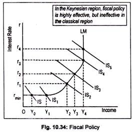
In Fig. 10.34, the IS curve intersects the LM curve at its horizontal portion (i.e., liquidity trap region). In this region, as the IS curve shifts from IS to IS₁, the equilibrium level of income rises from OY₀ to OY₁. Thus, fiscal policy is completely effective in stimulating aggregate income in the depressionary phase without having any effect on interest rate.

Secondly, in the classical range, fiscal policy is completely ineffective since it fails to stimulate aggregate demand and, hence, aggregate income. Fig. 10.34 says that the increased government expenditure and/or decreased taxes shifts the IS curve in the clas­sical region (where the LM curve is vertical) from IS₄ to IS₅.

This causes equilibrium intersection to shift up. This results in an increase in the interest rate only from Or₃ to Or₄, keeping income level unchanged at OY₄.

Finally, fiscal policy is partly effective in the normal intermediate range where both interest rate and income rise. Fiscal measures that shift the IS curve from IS₂ to IS₃, in the section between Keynesian and classical section, called, intermediate section, raises the level of income from OY₂ to OY₃ and the rate of interest from Or₁ to Or₂.

Thus, fiscal policy is found to have a degree of effectiveness in this region. It may be concluded that, in general, fiscal policy becomes more effective the closer the IS-LM intersection or equilibrium lies to the Keynesian or liquidity trap region and less effective the closer the equilibrium point resides to the classical region.

Thus, fiscal policy may be employed in depression years. This is the Keynesian argument. It is argued that these results con­cerning monetary policy are the opposites of the results obtained under fiscal policy regime.

Thus, one can conclude that the effective­ness of monetary policy depends on:

(i) The interest-elasticity of the demand for money, and

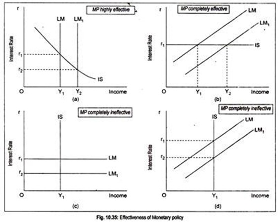
(ii) The interest elasticity of investment. These two aspects can be illustrated in terms of Fig 10.35.

If the LM curve is vertical (pure classical case), monetary policy becomes highly effective in raising equilibrium income [Fig. 10.35(a)]. Consequent upon an increase in money supply, the LM curve shifts from LM to LM₁. Equilibrium interest rate now declines from Or₁ to Or₂ and equilibrium income rises from OY₁ to OY₂.

The biggest effect of monetary policy can be felt if the IS curve is perfectly elastic [Fig. 10.35(b)], Note that, following a shift in the LM curve from LM to LM₁, national income rises from OY_: to OY₂ without influencing the interest rate that remains at Or₁.

On the other hand, if the LM curve is horizontal (pure Keynesian range) and if the IS curve is vertical, monetary policy becomes ineffective completely [Figs. 10.35(c) and (d)]. Fig. 10.35(c) says that a downward shift in the horizontal LM curve from LM to LM_X along with the vertical IS curve, income remains unchanged at OY1 while r declines to Or₂.

Thus, monetary policy does not have any influence in stimulating an economy in depression. Again, monetary policy fails to boost income/output of an economy if the positive sloping LM curve shifts from LM to LM₁, though interest rate declines from Or₁ to Or₂ following an increase in money supply.

Likewise, the effectiveness of fiscal policy depends on the slopes of the IS curve and the LM curve. The more interest-inelastic is the investment, the more effective is fiscal policy [Fig. 10.36(b)]. Likewise, the flatter the LM curve, greater is the effectiveness of fiscal policy [Fig. 10.36(c)]. Fiscal policy is completely ineffective in Fig. 10.36 a).