Law of Demand: Schedule, Curve, Function, Assumptions and Exception

The law of demand describes the relationship between the quantity demanded and the price of a product.

It states that the demand for a product decreases with increase in its price and vice versa, while other factors are at constant.

Therefore, there is an inverse relationship between the price and quantity demanded of a product.

“The greater the amount to be sold, the smaller must be the price at which it is offered in order that it may find purchasers; or in other words, the amount demanded increases with a fall in price and diminishes with a rise in price”-Marshall.

Some of the definitions of law of demand given by different authors are as follows:

According to Robertson, “Other things being equal, the lower the price at which a thing is offered, the more a man will be prepared to buy it.”

In the words of Marshall, “The greater the amount to be sold, the smaller must be the price at which it is offered in order that it may find purchasers; or in other words, the amount demanded increases with a fall in price and diminishes with a rise in price.”

According to Ferguson, “Law of Demand, the quantity demanded varies inversely with price.”

Demand is a dependent variable, while price is an independent variable.

Therefore, demand is a function of price and can be expressed as follows:

D = f(P)

Where

D= Demand

P= Price

f = Functional Relationship

In the law of demand, other factors of demand (except price) should be kept constant as the demand is subject to various influences. If all the factors would be allowed to vary at the same time, this may counteract the law. The law of demand can be understood with the help of certain concepts, such as demand schedule, demand curve, and demand function.

Demand Schedule:

Demand schedule refers to a tabular representation of the relationship between price and quantity demanded. It demonstrates the quantity of a product demanded by an individual or a group of individuals at specified price and time.

Demand schedule can be categorized into two types, which are shown in Figure-2:

The two types of demand schedules (as shown in Figure-2) are explained as follows:

i. Individual Demand Schedule:

Refers to a tabular representation of quantity of products demanded by an individual at different prices and time.

Table-1 shows the individual demand schedule of product a purchased by Mr. Ram:

Following are the characteristics of individual demand schedule:

a. Demonstrates the effect of changing price on the buying behavior of customers rather than change in the demand for a product

b. Expresses the disparity in demand with the difference in the product’s price

c. Represents that at higher prices the quantity demanded reduces and vice versa

ii. Market Demand Schedule:

Shows a tabular representation of quantity demanded in aggregate by individuals at different prices and time. Therefore, it demonstrates the demand of a product in the market at different prices. The market demand schedule can be derived by aggregating the individual demand schedules.

Table-2 represents the market demand schedule prepared through the individual demand schedule of three individuals:

Market demand schedule also demonstrates an inverse relation between the quantity demanded and price of a product.

Demand Curve:

Demand curve shows a graphical representation of demand schedule. It can be made by plotting price and quantity demanded on a graph. In demand curve, price is represented on Y-axis, while quantity demanded is represented on X-axis on the graph. R.G Lipsey has defined demand curve as “the curve which shows the relationship between the price of a commodity and the amount of that commodity the consumer wishes to purchase is called Demand Curve.”

Demand curve can be of two types, namely, individual demand curve and market demand curve. Individual demand curve is the graphical representation of individual demand schedule, while market demand curve is the representation of market demand schedule.

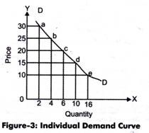
Figure-3 shows the individual demand curve for the individual demand schedule (represented in Table-1):

In Figure-3 points a, b, c, d, and e demonstrates the relationship between price and quantity demanded at different price levels. By joining these points, we have obtained a curve, DD, which is termed as the individual demand curve. The slope of an individual demand curve is downward from left to right that indicates the inverse relationship of demand with price.

Let us understand the individual demand curve with the help of an example.

Prepare a demand curve for the individual demand schedule of product X.

Solution:

The individual demand curve for the demand schedule of X (represented in Table-3) is shown in Figure-4:

In Figure-4, the DD curve represents the individual demand curve of product X.

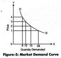
Market demand curve can be obtained by adding market demand schedules. Figure-5 shows the market demand curve for the individual demand schedules (represented in Table-2):

The market demand curve also represents an inverse relationship between the quantity demanded and price of a product.

Let us understand the market demand curve with the help of an example.

Example-2:

Ram, Shyam, Sharad, and Ghanshyam are the four consumers of product P. The individual demand schedules for product P by the four consumers at different price levels is represented in Table-4:

Determine the market demand curve for product P and prepare a market demand curve for product P.

Solution:

The market demand for product P can be determined by adding the individual demand schedules, as shown in Table-5:

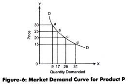
The market demand curve for product P is shown in Figure-6:

In Figure-6, the DD curve represents the demand curve of product P.

Demand Function:

A function can be defined as a mathematical expression that states a relationship between two or more variables containing cause and effect relationship. Similarly, demand function refers to the relationship between the quantity demanded (dependent variable) and the determinants of demand for a product (independent variables). In other words, demand function states the influence of various factors of demand, such as price, customer’s income and habits, and standard of living, on the demand of a product.

In the short run, the demand function states the relationship between the aggregate demand of a product and the price of the product, while keeping other determinants of demand at constant.

In such a case, the demand function can be expressed as follows:

Dx = f (Px)

Where, Dx= dependent variable

Px = independent variable

It can be interpreted from the preceding equation that quantity demanded (Dx) is the function of price (Px) for product X. This states that if there is any change in the price of product X, then the demand of product X would also show changes. However, the demand function does not interpret the amount of change produced in demand due to change in the price of the commodity.

Therefore, to understand the quantitative relationship between demand and price of a commodity, we use the following equation:

Dx = a – b (Px)

Where a = constant (represents total demand at zero price)

b = ∆D/∆P (constant, which represents the change in Dx produced by Px)

On the other hand, in the long run, demand function shows a relationship between the aggregate demand of a product and a number of determinants of demand, such as price, consumer’s income, standard of living, and price of substitutes.

On the basis of time period, the demand function has been classified as follows:

i. Linear Demand Function:

Refers to the demand function in which the change in dependent variable remains constant for a unit change in the independent variable, regardless the level of the dependent variable. In the linear demand function, AD/AP is constant and the resultant demand curve is a straight line.

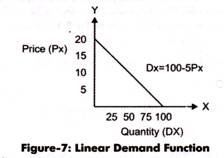
For example, if a=100 and b=5, then the demand function can be represented by the following equation:

Dx = 100 – 5 (Px)

With the help of the preceding equation, we can get the values of Dx by substituting the different values of Px, as shown in Table-6:

The linear demand function has been represented on graph (for Table-6) in Figure-7:

Price function can be obtained with the help of demand function by the following equation:

Px = a – Dx/ b

Px = a/b-(1 /b) Dx

Let us assume that a/b = a₁ and 1/b = b₁, then the price function would be:

Px = a₁ – b₁Dx

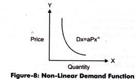
ii. Non-Linear Demand Function:

Refers to the demand function in which the dependent variable keeps changing with the change in the independent variable. In the non-linear demand function, the slope of the curve changes throughout the curve.

The equation for non-linear demand function is as follows:

Dx = a (Px)^-b and

Dx = (a/Px + c)-b

Where, a or b or c >0

The non-linear demand curve is shown in Figure-8:

iii. Multivariate or Dynamic Demand Function:

Expresses a relationship between a dependent variable, such as demand, and more than one independent variable, such as price and income. In the long-run, individual or market demand cannot be derived by using only one variable because other determinants are not constant and they do affect the demand for a product. In addition, in long-run, demand for a product can be determined by the composite demand of all the determinants affecting the demand for a product.

The multivariate demand function can be expressed as follows:

Dx = f (Px, M, Py, Pc, T, A)

Where, Px = Price

M = Consumer’s income

Py = Price of substitutes

Pc = Price of complementary goods

T = Consumer’s taste

A= Advertisement expenditure

If the relationship between the demand and its determinants is a straight or linear line, then demand function can be expressed as follows:

Dx = a + b Px + cM + dPy + ePc + g T + jA

Where, a = constant and b, c, d, e, g, and j = coefficients of relation between demand and its determinants

Example-3:

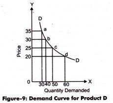
XYZ Organization has launched product D at the price of Rs. 20 per unit. With the increasing demand of product D, its price has reached to Rs. 25. The change in demand for the product is noticed to be 10 per week. After that, the price continuously with the increase in demand at the same rate and has reached to Rs. 35.

Determine the following for product D (taking a = 100):

i. Demand Function Equation

ii. Demand Schedule

iii. Demand Curve

Solution:

i. The demand function for product D can be expressed as follows:

D_D= a – b (Pd)

Where, a = 20

b = ∆D/∆P

b= 10/5

b = 2

Therefore, the demand function would be:

D_D= 20 – 2 (P_D)

ii. The demand schedule for product D is shown in Table-7:

iii. The demand curve for product D is shown in Figure-9:

Assumptions in Law of Demand:

The law of demand studies the change in demand with relation to change in price. In other words, the main assumption of law of demand is that it studies the effect of price on demand of a product, while keeping other determinants of demand at constant.

However there are certain assumptions underlying the law of demand, which are as follows:

i. Assumes that the consumer’s income remains same. If the income of an individual increases, the demand for products by him/her also increases, which is against the law of demand. Therefore, the income of consumer should not change.

ii. Assumes that the preferences of consumer remain same.

iii. Considers that the fashion does not show any changes, because if fashion changes, then people would not purchase the products that are out of fashion.

iv. Assumes that there would be no change in the age structure, size, and sex ratio of population. This is because if population size increases, then the number of buyers increases, which, in turn, affect the demand for a product directly.

v. Restricts the innovation and new varieties of products in the market, which can affect the demand for the existing product.

vi. Restricts changes in the distribution of income.

vii. Avoids any type of change fiscal policies of the government of a nation, which reduces the effect of taxation on the demand of product.

Apart from the aforementioned points, the law of demand assumes that the world is static and people consume products in the market at a fixed rate and price. These assumptions are not valid in the changing world.

Exception to Law of Demand:

Till now, we have studied that there is an inverse relationship between demand and price of a product. The universal law of demand states that the increase in the price of a product would decrease the demand for that product and vice versa.

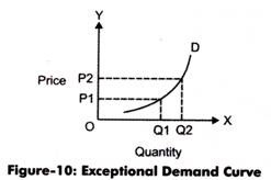
However, there are certain exceptions that with a fall in price, the demand also falls and there is an increase in demand with increase in price. This situation is paradoxical in nature and regarded as exception to the law of demand. In simple words, exception to law o demand refers to conditions where the law of demand is not applicable. In case of exceptions, demand curve shows an upward slope and referred as exceptional demand curve.

Exceptional demand curve is shown in Figure-10:

In Figure-10, D represents the demand curve in which OP1 is the price, and OQ1 is the initial demand. When the price rises from OP1 to OP2, then the demand also rises from OQ1 to OQ2. This implies that if the price of a product increases its demand also increases, which constitutes an exception to law of demand.

Certain cases that are exceptions to the law of demand are as follows:

i. Giffen Paradox:

Refer to one of the major criticism of law of demand. Giffin Paradox was given by Sir Robert Giffen, who classified goods into two types, inferior goods and superior goods, generally called Giffen goods. The inferior goods are those whose demand decreases with increase in consumer’s income, such as cheap potatoes and vegetable ghee.

These goods are of low quality; therefore, the demand for these goods decreases with increase in consumer’s income. In addition, if the price of these goods increases, then the demand for these goods increases assuming that the high price good would be of good quality tor example, coffee is considered as superior and tea as inferior. In case tile price of both of these goods increases the consumers would increase the demand of tea to satisfy their need by paying tile same amount.

ii. Necessity Goods:

Refer to goods that are considered as essential for consumer. The demand of necessity goods does not increase or decrease with increase or decrease in their prices. For example, salt is a necessity good whose consumption cannot be increased in case its price decreases. In such a scenario, the law of demand is not applicable.

iii. Prestige Goods:

Refers to goods that are perceived as a status symbol, such as diamond and Johny Walker Scotch Whisky. The demand for these goods remains same in case of increase or decrease in their price. In such a case, the law of demand is not applicable.

iv. Speculation:

Refers to an assumption of consumers about the change in prices of a product in future. If the price of a product IS expected to rise in future, then the demand for the product increases in the present situation. However, this is against the law of demand.

v. Psychologically Bias Customers:

Refer to one of the important exceptions to the law of demand. Different customers have different perceptions about the price of a product. Some customers have perceptions that low price means bad quality of a particular product, which is not true in all cases. Therefore, if there is a fall in the price of a product, then the demand for that product decreases automatically.

vi. Brand Loyalty:

Refers to the preference of a consumer towards a particular brand. Consumers do not prefer to change a brand with increase in the price of that brand. For example, if a consumer prefers, to wear Levi’s jeans, he would continue to purchase it, irrespective of increase in its price. In such a situation, the law of demand cannot be applied.

vii. Emergency Situations:

Refers to a condition for which the law of demand is not applicable. In emergencies, such as war flood, earthquake, and famine, the availability of goods become scarce and uncertain. Therefore, in such situations, consumer.’ prefer to store a large quantity of goods, regardless of their prices.