Average Cost and Marginal Cost (With Diagrams)

The relationship between average cost and marginal cost can also be studied in the context of laws of return.

It can be explained as under:

(i) Law of Increasing Returns or the Law of Diminishing Costs:

When a firm produces under the law of increasing returns, it means that as it employs more and more factors of production, its output increases at an increasing rate.

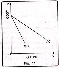
In such a situation both the average cost and marginal cost slope downward, but the downward slope of MC curve is more than that of AC curve.

From Figure 11 it becomes clear that when due to the operation of the law of increasing returns, average cost falls, marginal cost also falls. The fall in marginal cost is much more than the average cost, so the marginal cost remains below the average cost.

 

(ii) Law of Diminishing Returns or Increasing Costs:

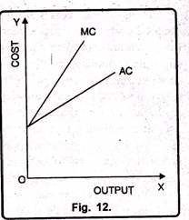
If a firm operates under the law of diminishing returns, it means its output increases at diminishing rate as it employs more and more units of factors of production. In this case, if AC increases MC also increases. The increase in MC will be much more than the increase in AC. It can be shown with the help of figure 12. The Figure 12 depicts that as AC increases MC also increases at a faster rate than the AC. Therefore, the curve MC remains above the curve AC.

(iii) Law of Constant Returns or Constant Costs:

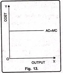
According to the law of constant returns when a firm employs more and more factors, output increases at a constant rate. Therefore, the average cost curve as well as marginal cost curve remains parallel to horizontal axis. This can be made clear with the help of diagram 13. In the diagram 13 output has been measured on OX- axis while costs on OY-axis. Here, we see that AC = MC and both are parallel to X-axis.

 

 

Relationship of Different Cost Curves in Short Period:

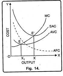
In Figure, the relationship between different cost curves can be explained with the help of figure 14. In Fig. 14 AFC is the average fixed cost curve which slopes downward. It indicates that as production increases, AFC goes on falling. In the beginning, it slopes steeply but later on rate of fall slows down. AVC is the average variable cost. It falls up to point E and then rises upward. SAC is the short run average cost curve having U-shape. The minimum point E of AVC occurs earlier than the minimum point E’ of SAC. MC passes from the minimum points of both AVC and SAC through the points E and E’ respectively.

Costs in Long Run Period:

Long-run is a period in which there is sufficient time to alter the equipment and the scale or organization with a view to produce different quantities of output. In other words, if we want to change output, it can be done by changing all the factors. It is due to the reason that in the long-run, all the factors are variable.

According to Koutsoyiannis, “In the long-run, all the factors of production are assumed to be variable.” In the same fashion Leftwich has defined the long-period as, “It will be helpful to think of the long run situations into any one in which the firm can move.”

 

Long Run Total Cost:

According to Leibhafasky, “The long run total cost of production is the least possible cost of producing any given level of output when all inputs are variable.”

Long run total cost is always less than or equal to short run total cost, but it is never more than short run total cost. Long run total cost curve represents the least cost of different quantities of output. Therefore, it is tangent to any given point, on short run total cost. In Fig. 15 three different types of long run total cost curves are shown. LTC₁ has been drawn on the assumption that as output is increased, cost at first rises at diminishing rate and then at increasing rate. LTC₁ has been drawn on the assumption that increase in output is followed by rise in cost at constant rate.

LTC₃ has been drawn on the assumption that as output increases, cost rises at diminishing rate. Long run cost curve always begins from the point of origin while short run cost curve begins from any point on OY-axis. It means that all costs in long run are variable when quantity of output is zero, total costs also reduced to zero.

Long-Run Average Cost Curve:

Long-run average cost is the long run total cost divided by the level of output.

LAC = LTC / Q

According to Robert Awh, “The long run average cost curve shows the lowest average cost of producing output when all inputs can be varied freely.”

Similarly, J.S. Bain has defined the long-run average cost as, “The long-run average cost curve shows for each possible output, the lowest cost of producing that output in the long run.” Moreover, in the long-run, each firm can make use of different sizes of plants.

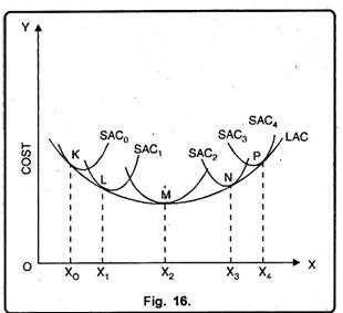
A given level of output can be had from a special plant to which it is appropriated. If, such a plant is put to operation, goods will be produced at the lowest average cost. Thus, a rational producer in the long- run will choose to produce with the help of such a plant. Now, the question is how to find out this long-run average cost curve. The answer is very simple. We can derive the LAC from the short-run average cost curves.

In Figure 16 long-run average cost has been shown. The long- run average cost curve is tangent to different short run average cost curves. In order to produce OX₀ level of output, the corresponding point on LAC is K at which it 1S tangent to SAC₀. Therefore, if a firm is willing to produce OX₀ level of output, it will construct a plant corresponding to SAC₀ and will operate on this curve at point K.

Different Names of LAC:

LAC is also known by the following names:

(i) Envelope curve:

LAC is also known as envelope curve because it envelopes all the SAC curves. It indicates that LAC cannot exceed SAC. As in the long-run indivisible factors can be used to their full capacity, therefore, LAC curve will be surrounding the SAC. It will not cut SAC curves or rise upward.

(ii) Planning curve:

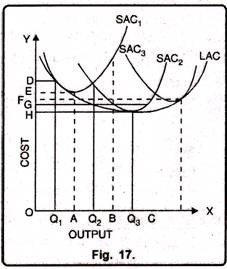
LAC is also known as planning curve. With its help, a firm can plan as to which plant; it should use to produce different quantities of output so that production is obtained at minimum cost. This fact can also be explained with the help of fig. 17.

In the Fig. 17, short-run average cost curves of all the three types of plants have been shown. If the firm has to produce OQ₁ output, it will select small plant. If it wants to produce OQ3 level of output, it will select the large output plant.

If the firm begins production with the small plant and demand for its product rises slowly, it will produce at minimum cost up to OA quantity of output. After OA amount of output its cost begins to rise. In case, demand for the product of the firm increases to OB then the firm will produce either with small or medium plant.

Relationship between LAC and SAC:

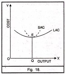
The relationship between LAC and SAC can be explained with the help of Fig. 18.

(1) Representation:

SAC represents the costs of a single plant, whereas LAC represents the costs of different plants.

(2) Shape:

Like SAC, LAC is also U-shaped but it is relatively flatter. The U-shape of LAC is less pronounced as compared to SAC. It indicates that in the long run, increase or decrease in costs is relatively less. It is so because LAC represents the minimum average cost of different quantities of output so there exists less possibilities of fluctuations.

(3) LAC does not Exceed SAC:

LAC cannot be more than SAC. It is so because LAC is tangent to SAC

(4) LAC Not Tangent to all SAC at their minimum points:

Except to one SAC curve, LAC is not tangent to SAC curve at their minimum point. It will be tangent to that SAC curve at its minimum point which coincides with the minimum point of LAC.

Long-Run Marginal Cost:

Long-run marginal cost shows the change in total cost due to the production of one more unit of commodity. According to Robert Awh, “Long-run marginal cost curve is that which shows the extra cost incurred in producing one more unit of output when all inputs can be changed.”

LMC = ∆LTC / ∆ Q

Where

LMC = Long run Marginal Cost

∆LTC = Change in Long-Run Total Cost

∆Q = Change in Output

Relation between LMC and LAC:

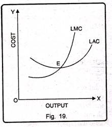
Generally, the relation between long-run marginal cost and long run average cost is similar to that of what it is in short run AC and MC. But the only difference in LAC and LMC is that long run marginal and average costs are more flatter than that of SAC and SMC. It is so because in the long run all factors are variable. It can be shown with the help of a figure 19.

 

In Figure 19 when LAC is falling, LMC also falls but the fall in LMC is greater than that of LAC. At a minimum point i.e. E, LMC is equal to LAC. In the same fashion when LAC raises LMC also rises. But the increase in LMC is more than the increase in LAC.

Relation between LMC and SMC:

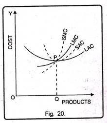
SMC refers to the effect on total cost due to the production of one more unit of output on account of change in variable factors. LMC refers to change in total cost due to production of one more or less unit of output due to change in all factors. When a firm selects a proper scale of plant in order to produce a given quantity of output then at this level of output short run and long run marginal cost curves are equal. This can be shown with the help of fig. 20.

In Fig. 20, OQ is the optimum level of output SMC = LMC. If output is less than the optimum level OQ, then SMC will be less while LMC will be relatively more. On the other hand, if output is more than the optimum level, SMC will be more while LMC will be relatively less.

Modern Theory of Cost Curves:

Modern theories of costs have been provided by economists like Stigler, Andrews, Sargent, Florence and Friedman etc. According to traditional theory of costs, costs are of U-shape. But according to modern economists, in real life cost curves are L-shaped.

Modern Theory of Short Run Cost Curves:

Like traditional theory modern theory also studies four types of short run cost curves as Average fixed cost, Average variable cost, average cost & marginal cost.

Average Fixed Costs:

This is the cost of indirect factors, that is, the cost of the physical and personal organization of the firm.

The fixed costs include costs on account of:

(1) The salaries and other expenses of administrative staff;

(2) Salaries of staff involved directly in production but paid on a fixed-term basis;

(3) The depreciation of machinery;

(4) Expenses on account of the maintenance of the factory-buildings;

(5) Expenses connected with the maintenance of land on which the plant is installed and operated.

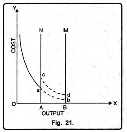
The average fixed cost curve, under these circumstances will be as shown in Fig. 21. The firm has some largest capacity units of machinery which set an absolute limit to expansion of output in the short run. This is indicated by boundary line M in the diagram.

The firm also has some small sized machinery which set a limit to expansion. This is shown by the boundary line N.N, however, is not an absolute limit because the firm can expand its short run output up to M by paying overtime to labour for working longer hours. In this case, the AFC is shown by the dotted line ab. The firm can also expand output by purchasing some additional small-sized machinery. In this case, the AFC shifts upwards and starts falling again, as shown by the dotted line CD.

 

Average Variable Cost:

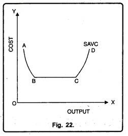
In modern economics, the average variable cost includes wages of labour employed, cost of raw- material, and running expenses of machinery. The short run average variable cost curve in modern-micro economic theory is saucer-shaped, that is, it is broadly U-shaped but has a flat stretch over a range of output. This flat stretch represents the built-in reserve capacity of the plant. Over this flat stretch, the SAVC is equal to the MC, both being constant per unit of output. To the left of the flat stretch, MC lies below the SAVC, while to the right of the flat stretch; marginal cost rises above the SAVC.

The falling portion of the SAVC shows reduction in costs due to better utilization of the fixed factor like machinery and also due to improvement in the skill and efficiency of labour. Better efficiency of labour helps in reducing wastage of raw-material and achieving better utilization of the whole plant. On the other hand, rising portion of the SAVC curve indicates declining labour efficiency due to longer hours of work, rising costs due to payment of over-time wages, frequent breakdown of machinery, and wastage of raw-materials.

This has been shown in Fig. 22.

Short Run Average Cost Curve:

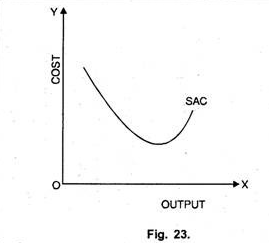
According to modern economists, short run average cost curve is continuously falling up to a given level of output. This given level of output represents reserved capacity output. Thereafter, average cost curve rising upward meaning thereby that average cost will rise rapidly if output is increased beyond reserved capacity. This is shown with the help of figure 23.

 

Short Run Marginal Cost Curve:

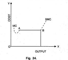
In the initial stages, SMC, to modem economist’s falls, from point A to B it becomes horizontal. Moreover, from A to B marginal cost is equal to average variable-cost. In this situation, production takes place under reserved capacity as shown in Figure 24.