Linear Programming (Explained With Diagrams)

I. General Notes:

Linear programming is a recently devised technique for providing specific numerical solutions of problems which earlier could be solved only in vague qualitative terms by using the apparatus of the general theory of the firm.

Linear programming has thus helped to bridge the gap between abstract economic theory and managerial decision-making in practice.

The use of linear programming is expanding fast due to the use of computers which can quickly solve complex problems involving the optimal use of many resources which are given to the firm in any particular time and thus set con­straints on the firm’s choice. Linear programming can be considered as providing an operational method for dealing with economic relationships, which involve discontinuities. It is a specific approach within the general framework of economic theory.

The main similarities and differences between traditional economic analysis and linear programming may be outlined as follows. Both approaches show how economic agents (consumers or producers) reach optimal choices, how they do their planning or programming in order to attain maximum utility, maximum profit, minimum cost, etc. Neither economic theory nor linear programming say anything about the implementa­tion of the optimal plan or solution.

They simply derive the optimal solution in any particular situation. In that sense both approaches are ex ante methods aiming at helping the economic units to find the solution that attains their goal (utility maximisa­tion, profit maximisation, cost minimisation) given their resources (income or factor inputs) at any particular time.

However, in economic theory the optimal solution is usually shown in qualitative abstract terms, diagrams, or general mathematical symbols, while linear programming yields specific numerical solutions to the particular optimization problems.

Another difference between economic analysis and linear programming is that the relationships of economic theory are usually non-linear, depicted by curves (not straight lines), while in linear programming all relationships between the variables involved are assumed to be linear.

Methods of non-linear programming have recently been developed, but their exposition involves sophisticated mathematics and will not be attempted here. We will illustrate the use of linear programming by a simple example of a firm which has a given quantity of three factors of production with which it can produce two commodities, x and y. The problem of the firm, given its resources, is to choose the opti­mal product mix which maximises the firm’s profit.

II. Statement of the Linear Programming Problem:

Assume that a firm has the following quantities of factors of production

L = 400 units of labour (hours)

K = 300 units of capital (machine hours)

S = 1000 units of land (square feet)

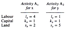
The firm can produce either commodity x or commodity y with the following available processes (activities)

In words, the production of one unit of x requires 4 hours of labour, 1 machine hour and 2 square feet of land. Similarly, the production of one unit of y requires 1 hour of labour, 1 machine hour and 5 square feet of land. Commodity x yields a unit profit of £2, and commodity y yields a unit profit of £1 .5.The goal of the firm is to choose the optimal product mix, that is, the mix that maximises its total profit.

The total profit function may be written as follows:

Z = 2X + 1 Y

where Z = total profit

X = quantity of commodity x (or level of Activity A₁)

Y = quantity of commodity y (or level of Activity A₂)

2 and 1 are the unit profits of the two commodities. The total profit function is called the objective function, because it expresses the objective of the firm, which in our par­ticular example is the maximisation of profit. In general, the objective function is the function which represents the goals of the economic agent.

The firm, in pursuing the maximisation of its objective function, has several con­straints. We distinguish two groups of constraints, technical (or functional) constraints, and non-negativity constraints. The technical constraints are set by the state of technology and the availability of factors of production.

There are as many technical constraints as the factors of production. They express the fact that the quantities of factors which will be absorbed in the production of the commodities cannot exceed the available quantities of these factors. Thus the technological constraints take the form of in­equalities.

In our example the technical constraints are the following three:

4X + 1 Y < 400

1x + 1Y < 300

2X + 5Y < 1000

where X and Y are the levels of commodities x and y (levels of utilisation of activities A₁ and A₂) and the integers on the left-hand side are the technical coefficients of pro­duction, that is, the factor inputs required for the production of one unit of the products x and y. The figures on the right-hand side are the resources that the firm has at it disposition. These inequality constraints state that the levels of X and Y in the optima product mix should not require more than the available quantities of the three re­sources.

The non-negativity constraints express the necessity that the levels of production of the commodities cannot be negative, since negative quantities do not make sense in economics. The level of production of any one commodity can either be zero or positive

X > 0

y > 0

Given the above information, the linear programming problem may formally be stated as follows:

Note that all the constraints take the form of inequalities. Thus the system cannot be solved with the usual methods of solution of simultaneous equations. The linear programming technique has been designed to deal with the solution of problems involving inequalities. Its basic approach is that of iteration the optimal solution is defined by examining the set of possible alternative solutions and eliminating gradually the suboptimal ones until the optimal is reached.

III. Determination of the Optimal Solution:

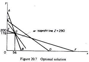
The optimal solution is found by the point of tangency of the frontier of the region of feasible solutions to the highest possible isoprofit curve. The optimal solution will be a point on the frontier of the region of all feasible solutions, because any point inside this region lies on a lower isoprofit line. It is clear that the optimal solution depends on the slope of the isoprofit lines, that is, on the ratio of the unit profits of the two commodities. In our example the optimal solution is point G in figure 20.7.

At this point the product mix is 178 units of y and 56 units of x, and the maximum profit amounts to £290, as can be verified from the profit function

Z = 2X + 1Y = 2(56) + 1(178) = 290

If the slope of the isoprofit line is equal to the slope of any one of the boundary lines which define the region of the feasible solutions, there is no unique optimal solution to the linear programming problem. For example, if π_x/π_y = l_x/l_y (= slope of AB which is the boundary for the factor ‘labour’ all the points on the segment GB will be optimal solutions.

Similarly, if π_x/π_y — s_x/s_y (= slope of EF which is the boundary for the factor ‘land’) all the points on the segment EG of the production-possibility frontier will be optimal solutions. From the above discussion it should be obvious that a unique optimal solution exists if the slope of the line representing the objective function has a value lying within the range set by the slopes of the boundary lines which denote the technical restrictions of the linear programming problem.

We may generalize the above procedure for the determination of the optimal solution as follows:

Step 1:

Write the technical inequalities in the form of equalities and solve them for Y

l₁x + / l₂y = L

k₁X + k₂Y = K

s₁X + s₂Y =S

Solving these equations for Y we obtain the equations of the three boundary lines:

The equation of boundary L is

The slope of the L boundary is

∂Y/∂X = – l₁ / l₂

We may draw the L boundary by assigning various values to X and plotting the re­sulting points on a graph. (The value of L is given.)

The equation of the boundary K is

The slope of the K boundary is

∂Y/∂X = – k₁ / k₂

We may draw the K boundary by assigning various values to X (given the value of K) and plotting the resulting points on a graph.

The equation of the boundary S is

The slope of the S boundary is

∂Y/∂X = – s₁ / s₂

We may draw the S boundary by assigning different values to X (given the quantity of S) and plotting the resulting points on a graph.

Step 2:

Determine the region of feasible solutions. This is the area within all the boundaries set by the technical restrictions. Only the parts of the areas below the individual boundary lines that coincide, when the various graphs (of Step 1) are com­bined, do satisfy all the constraints.

Step 3:

Define the isoprofit lines by solving the profit equation for Y

The set of isoprofit lines can be drawn by assigning different values to Z and to X.

Step 4:

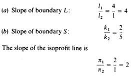
Define the optimal solution by comparing the slope of the isoprofit line with the slopes of the boundary lines that define the region of feasible solutions. Since all lines have negative slopes we can ignore their signs when doing the comparison. In our example only two boundary lines define the region of feasible solutions. (The factor K does not set any limit to the choice of the firm, given the other factors L and S.)

The slopes of the boundary lines are we conclude that there is a unique solution, and that this optimal solution is defined by the intersection of the two boundary lines that define the region of feasible solutions.

IV. The Simplex Method:

When the variables whose values must be determined from the linear programming method are more than two, the graphical solution is difficult or impossible because we need multidimensional diagrams. The following iterative method for reaching the optimal solution, which is called the simplex method, may be used.

We will illustrate the simplex method by using the following example.

Assume that a firm can produce five commodities, x₁, x₂, …, x₅, with three factors of production F₁, F₂, F₃.

The available quantities of factors are:

F₁ = 100 units of labour

F₂ = 80 units of capital

F₃ = 150 units of land

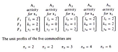
The known methods of production (processes or activities) for each product are

The firm wants to choose the product mix that maximises its total profit z. Let us denote the levels of production of the five commodities by the capital X letter with the appropriate subscript.

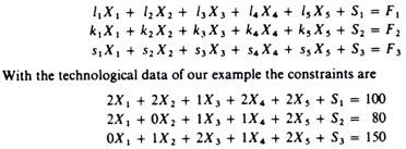
With the above information we can state the linear programming problem formally as follows:

Substituting the technical information of our example we:

To overcome the difficulties created by the inequalities in the constraints we transform the technical constraints into equalities by introducing into each one of them a variable, called the ‘slack variable\ which will show the unutilised units of the corresponding factor of production. Clearly there will be as many slack variables as there are factors of production. It is assumed that unutilized factors have zero profitability (neither profit nor loss).

With the introduction of the slack variables the constraints become:

a. The Iterative Procedure

Iteration I:

We start from any one feasible solution, find its profitability and consider whether it yields maximum profit as compared with other feasible solutions. The levels of output and of unused factors in any one solution form a basis. The easiest way to begin the iterations is to start from the basis that shows zero production, that is, it includes the three slack activities with values equal to the available quantities of the three factors of production, since with no production all the factors are unutilized. Thus the initial solution (Basis I) is the origin, where all levels of output are zero

X₁ = X₂ = X₃ = X₄ = X₅ = 0

and all inputs are unemployed, so that

S₁ = F₁ = 100

5₂ = F₂ = 80

5₃ = F₃ = 150

This is a feasible solution, because all the constraints are satisfied. Clearly it is not optimal, since profits are zero if there is no production

Z = 2(0) + 2(0) + 3(0) + 4(0) + 6(0) 4 0(S₁) + 0(S₂) + 0(S₃) = 0

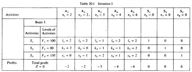
Before we proceed to find a better feasible solution we will present the first solution (Basis I) in a table (table 20.1).

In the first column we show the activities that are included in the solution (Basis), which is being examined, and their levels of utilisation. Basis I includes the slack activi­ties S₁, S₂, S₃, and their levels of utilisation are equal to the unused factors of produc­tion, 100 units of f₁, 80 units of f₂ and 150 units of f₃.

In the columns of the five productive activities we insert the inputs of the three factors of production which are required for the production of one unit of the cor­responding commodities.

In the columns of the slack activities we insert unity for the corresponding factor of production, and zero for all other factors.

In the last row of the table we insert the total profit (Z) of the Basis and the unit profits of the activities with a negative sign. This row (which we will call the ‘profit­ability row’) is crucial in the iterative procedure of the simplex method, because it shows which is the most profitable activity which should be introduced in the next iteration. When all the elements in this row become positive or zero we stop the itera­tions.

Positive elements in the ‘profitability row’ suggest that the introduction of the corresponding activities in the Basis will lead to a decrease in the total profit. Zero elements in the ‘profitability row’ (in the columns of the productive activities A_1, … , A₅) imply that there are other optimal solutions which yield the same total profit. Thus when the elements of the ‘profitability row’ (of the columns of the productive activities) are either positive or zero we stop (usually) the iterations since an optimal solution has been reached.

Iteration II:

We must find the incoming activity and the outgoing activity, that is the activity which we must introduce in the Basis and the one that will be replaced.

As incoming activity we choose the one with the highest unit profit, that is, the activity with the largest negative element in the ‘profitability row’. In our example the most profitable activity is A₅.

The outgoing activity is found by dividing each activity level in the first Basis (F₁, F₂, and F₃ in our example) by the relevant input coefficient of the incoming activity, and choosing to replace the activity of the old Basis for which the ratio is the smallest. In our example we have

The smallest ratio is F₂/k₅, hence the outgoing activity is S₂. The new Basis will include the activities S₁, A₅ and S₃. We replace the slack activity whose ratio is the smallest, because the corresponding resource will be the first to be exhausted as we expand the production of commodity x₅ (produced by the incoming activity).

Our next step is to find the elements of the new iteration table.

The following steps are involved in this process:

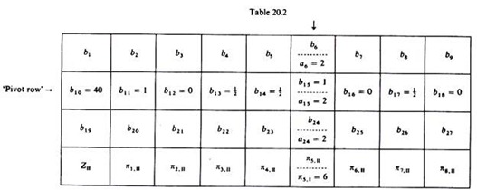
1. We define the pivot element, which is the element at the intersection of the in­coming and the outgoing activities. In our example the pivot element is 2, at the inter­section of A₅ and S₂.

2. We find the elements of the pivot row, that is, the row that will be occupied by the incoming activity, taking the place of the outgoing activity. The elements of the pivot row are found by dividing the elements of the original row (of the outgoing activity) by the pivot element (2 in our example). The elements of the pivot row are the elements of the incoming activity (A₅) in the new iteration table.

In our example the elements of the pivot row are:

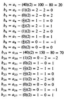
3. Any other element in the second iteration table b_i is found by subtracting from the corresponding original element a, (in the first iteration table) the product of the element of the pivot row which is in the same column as a, multiplied by the element of the in­coming activity which is in the same row as a_i.

The computations are shown in table 20.2. The crucial data required at this stage are the elements of the pivot row (b₁₀, b_{1 1} …, b₁₈) and the elements of the column of the outgoing activity (a₆ = 2, a₁₅ = 2, a₂₄ = 2).

The elements of the first and third rows of the second iteration table are:

4. The total profit of the new solution (Z_ll) is found by multiplying the levels of the activities in this Basis by their unit profits

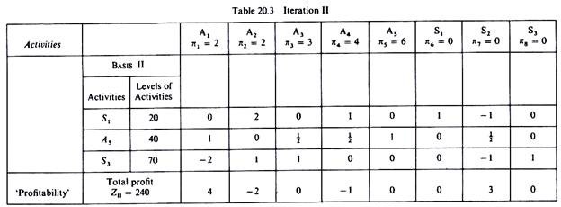
Z_II = π₆(S₁) + π₅(/A₅) + π₈(S₃) = (20) (0) + (40) (6) + (70)(0) = 240

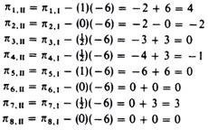
5. The elements of the ‘profitability row’ are estimated in the same way as the other elements of the second iteration table. That is, from the initial ‘profitability elements’ we subtract the product of the element of the pivot row (which is in the same column as π_i.I) times the ‘profitability element’ of the incoming activity

We have now completed the computation of the elements of the second iteration. The results are shown in table 20.3.

S₁ = 20 A₅ = 40 S₃ = 70

It is clear that the second Basis is better than the initial solution, since it yields a total profit of 240 monetary units. However, so long as negative elements appear in the last row of the iteration table, we can further improve our solution (increase profits) by introducing into the basis the activity which has the largest negative ‘profitability element’.

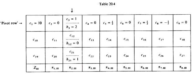
In our example activity a₂ which produces commodity x₂ will be the incoming activity in the new solution (Basis III). The outgoing activity is determined in the same way as in the previous iteration. That is, we divide the slack activities in Basis II by the corresponding elements in the column of the incoming activity (A₂) and we drop out the activity with the smallest ratio. In our example we have

_20/2 = 10 and _70/1 = 70

Since (20/2) < (70/1) the outgoing activity at this iteration is 5,. (Table 20.4.)

Before we proceed with the computations of the third iteration it is useful to indicate the implications of the simplex criterion. This criterion serves in defining whether the optimal solution has been reached, or whether a further improvement can be achieved by additional iterations.

The simplex criterion may be summarised in the following propositions:

If one or more elements in the ‘profitability row’ are negative, further improvement of the solution is possible, and the iterations should continue, unless all the elements of the incoming activity are positive or zero. In this case we infer that the problem has no solution or it has not been correctly stated.

If all the elements in the ‘profitability row’ are positive or zero, the Basis in this table is an optimal solution, and further iterations are (usually) not required. The inclusion in the Basis of activities with positive ‘profitability elements’ reduces the total profit of the firm, and hence such activities should not be considered as a means for improving the solution.

If some of the productive activities have zero ‘profitability elements’ in the final table, there is more than one optimal solution. If we introduce in the Basis an activity with zero ‘profitability’, the total profit is not affected.

Iteration III:

The last row of the second iteration table contains negative elements and hence the solution can be improved. The incoming activity is the one with the greatest negative ‘profitability element’ (A₂ in our example), and the outgoing activity is S₁ which has the smallest ratio (S₁/2 = level of S₁ in Basis II divided by the corresponding element of the column of the incoming activity).

Having defined the incoming and the outgoing activities, we repeat the computations of the second iteration:

1. The pivot element is 2, defined by the intersection of the incoming and the out­going activities.

2. The elements of the ‘pivot row’ are defined by the division of the elements of the outgoing activity into the pivot element. They are

_20/2 =10, _0/2 = 0, _2/2 = 1, _0/2 = 0, _{1/2, 0/2} = 0, _1/2, _-1/2, _0/2 = 0

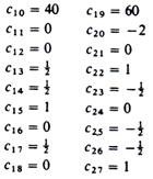
3. The remaining elements (c_i) of the third iteration table are found by subtracting from the corresponding elements of the second iteration table (b_i) the product of the element of the ‘pivot row’ (which is in the same column as b_i) times the element of the incoming activity (which is in the same row as b_i).

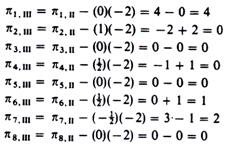
The values of the elements of the third iteration are:

4. The total profit of the Basis III is found by adding the products of the levels of the activities included in this basis times their corresponding unit profits (as given in the objective function)

Z_III = (10) (2) + (40) (6) + (60) (0) = 260

This is higher than the profit of the previous solution (Z_II = 240).

5. The elements of the ‘profitability row’ of the third iteration are computed as in the second iteration

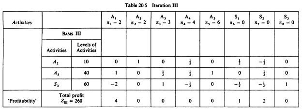
Thus we have completed the computations of the elements of the third Basis. The results are shown in table 20.5.

Using the propositions of the simplex criterion we observe the following. All the elements in the last row (‘profitability row’) are either positive or zero. This implies that this table contains an optimal solution.

The activities of this Basis are:

A₂ = 10 units of commodity x₂

A₅ — 40 units of commodity x₅

S₃ = 60 units of unutilized factor F₃

The total profit of this optimal solution is 260 monetary units. Given that there are zeros in the last row (and in the columns of the productive activities), we infer that the above solution is not unique. That is, there are other optimal solutions (which include the productive activities with zero ‘profitability elements’). These alternative optimal solutions of course yield the same total profit. Since we have found an optimal solution we will not proceed with further iterations. However, there are cases in which the location of additional optimal solutions might be useful.

V. The Dual Problem and Shadow Prices:

The basic problem whose solution is attempted by the linear programming technique is called the primal problem. To each primal problem corresponds a dual problem, which yields additional information to the decision-maker. The nature of the dual problem depends on the primal problem. If the primal problem is a maximisation problem, its dual is a minimisation problem. Similarly, if the primal is a minimisation problem its dual is a maximisation problem.

The detailed examination of the dual problem is beyond the scope of this book. We will concentrate here on the dual problem of our earlier example of profit maximisation. The dual problem in this case is one of cost minimisation, and from its solution we derive the shadow prices of the factors of production used by the firm.

The dual problem may be solved independently from its primal by a similar procedure to the one de­scribed above. However, the values obtained from the solution of the dual are also obtained as a by-product from the last iteration of the primal, which yields the optimal solution.

In our example the shadow prices of the three factors of production are the elements appearing in the last three cells of the ‘profitability row” of table 20.5.)If the optimal solution contains a slack activity showing that some quantity of the corre­sponding factor remains unemployed, this factor has a shadow price equal to zero.

If the factors are fully employed, their shadow prices are positive. In our example the shadow prices of the factor labour (F₁) and the factor capital (F₂), which are fully employed in the optimal solution, appear as positive and equal to 1 and 2 monetary units respectively. The shadow price of the factor land (F₃) is zero, because this factor is not fully employed in the optimal solution.

The shadow prices of the factors are the imputed costs or opportunity costs of the factors for the particular firm. As such they are crucial indicators for the expansion of the firm. They show which factors are bottlenecks to the further expansion of the firm, since these factors will appear with a positive shadow price (opportunity cost) in the optimal solution.

Furthermore the shadow prices of the resources can be compared with their market prices and help the entrepreneur decide whether it is profitable to hire additional units of these factors. The shadow price of a factor denotes by how much the profit of the firm will be increased if the firm employs an additional unit of this factor.

In our example we see that if the firm hired an additional unit of labour its profits would increase by 1 monetary unit. Similarly, if the firm employed an additional unit of capital its profit would rise by 2 monetary units. But in order to hire additional units of L and/or k the firm would have to pay their market price (wage or rent of capital).

Thus, if the shadow price of a factor is larger than its market price, it would pay the firm to increase its employment of that factor, since the firm’s net profit would increase. Obviously the shadow prices, whose values are estimated from the linear programming technique, are of great practical importance to the firm.