The graphical solution is simple when the problem can be presented on two- dimensional diagrams, as in our simple example.
When there are more than two variables the graphical solution becomes extremely complicated or impossible to draw.
The graphical solution involves two steps.
Firstly, the graphical determination of the region of feasible solutions.
ADVERTISEMENTS:
Secondly, the graphical presentation of the objective functions.
A. Graphical Determination of the Region of Feasible Solutions:
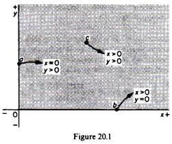
A solution is called feasible when it satisfies all the constraints. The non-negativity constraints in our example are shown graphically by the area of the positive quadrant of the usual orthogonal co-ordinate system (figure 20.1). Points on the horizontal axis denote that the production of y is zero, while the production of x is positive. That is, on the x-axis X > 0 and Y = 0.
Similarly, points on the y-axis denote that there is no production of x, while the production of y is positive. That is, on the y-axis X = 0 and Y > 0. Clearly points lying inside the two axes imply some production of both commodities (X > 0 and Y > 0). The shaded area in figure 20.1 and its boundaries (denoted by the two axes) represent the region in which the non- negativity constraints are satisfied.
ADVERTISEMENTS:
The complete determination of the region of feasible solutions requires in addition the determination of the boundaries or limits set by the technical (functional) constraints, that is, the availability of the factors of production and the given state of technology.
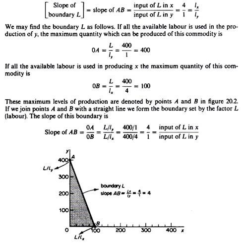
Boundary set by the factor ‘labour. This is defined by a straight line whose slope is the ratio of the labour inputs in the production of the two commodities. Thus if we denote the boundary set by labour with the letter L, we have
The feasible region of production of x and y defined by the availability of labour (L) is the shaded area OAB in figure 20.2.
ADVERTISEMENTS:
Boundary set by the factor capital:
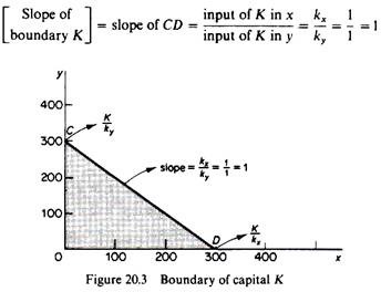
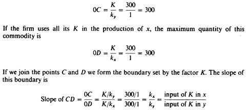
In a similar way we may derive the boundary (or limit) set to the production possibilities of the firm by the available quantity of the factor capital (K). The boundary of K will be a straight line (CD in figure 20.3) whose slope is the ratio of the capital inputs in the production of the two commodities.
In our example the boundary of capital can be determined as follows. If the firm uses all the available units of K in the production of y, the maximum quantity of this commodity is
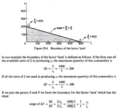
Boundary set by the factor ‘land”. The boundary of the factor ‘land’ (S) is determined in the same way as the previous two boundaries. It is a straight line (EF in figure 20.4) whose slope is the ratio of the land inputs in the production of the two commodities
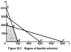
The region of feasible solutions of the firm is determined graphically if we superimpose the three diagrams showing the boundary-constraints set to the production possibilities of the firm by all the factors of production simultaneously.
ADVERTISEMENTS:
In figure 20.5 the region of feasible solutions is shown by the area 0EGB in which all the inequality constraints (technical and non-negativity constraints) are satisfied. Only combinations of x and y lying in this area and on its boundaries are feasible, given the availability of factors and the state of technology. Of all the feasible solutions only the ones lying on the frontier EGB are technically efficient. Thus the optimal solution must be one of the points on the frontier (EGB).
B. Graphical Determination of the Objective Function:
ADVERTISEMENTS:
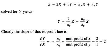
We said that among all the feasible solutions the firm will choose the one that maximises its objective function, that is, the product mix which yields the maximum profit. The objective function in our example may be presented graphically by isoprofit lines. We may construct an isoprofit line by solving the objective function for Y. Thus the profit function
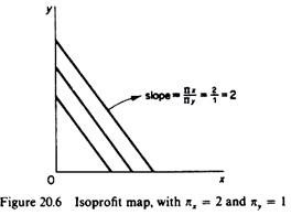
By assigning various values to the level of total profit (Z) we can compute the whole family of isoprofit lines (isoprofit map, figure 20.6). These lines have a negative slope and are parallel, given that the unit profits of the two commodities are assumed constant. The further away from the origin an iosprofit line is the greater the total profit it denotes.
