LM Curve: Subject Matter, Slope and Position (With Diagram)

Let us make an in-depth study of the LM Curve:- 1. Subject-Matter of the LM Curve 2. The Slope and Position of the LM Curve.

Subject-Matter of the LM Curve:

The demand for real money balances is found simply by adding together the transactions demand for money and the asset demand for money.

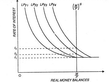
As the transactions demand for real money balances is an increasing function of real income, the total demand for real money balances can be shown as a function of the real rate of interest that shifts to the right as real income is increased. This is shown in figure 14.3 (a). As real income increases from Y₁ to Y₂, the demand for real money balances shifts from LPY₁ to LPY₂ and so on as income increases in real terms through Y₃ and Y₄.

Suppose that the economy is initially in an equilibrium position with real income as K₃ and the real interest rate at r₃. This equilibrium position for the money market is shown in Figure 14.3 (a). If conditions in the product market change, the level of real income being generated will change and equilibrium in the money market would be disturbed. For example, if real aggregate demand increases, real output from the product market will rise and the additional real income will increase demand for real money balances.

If this product market adjustment increases real income to Y₄, the demand for real balances curve will shift to the right to LPy₄ as shown in figure 14.3(a). The increased transaction demand for real money balances will generate an excess demand for real money balances at the old equilibrium rate of r₃. This excess demand for real money balances will induce adjustment in the money market.

Fig. 14. (a) Equilibrium in the money market  

Fig. 14.3 (b) Derivation of the LM curve  

The market real rate of interest will rise as individuals sell off some of their holdings of bonds and attempt to borrow the additional real money balances desired. The market real rate of interest will rise until the money market reaches the new equilibrium position at the real interest rate r₄. Different equilibrium positions in the money market for various levels of real income are shown in figure 14.3(a)

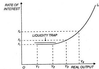
The relationship between levels of real income and the corresponding equilibrium real interest rates in the money market is called the LM curve. For the real income level Y₃ equilibrium between the demand for real money balances and the quantity of real balances supplied occurs at real interest rate r₃. When real income increases to Y₄ equilibrium in the money market occurs at real interest rate r₄.

The equilibrium positions in the money market for a given supply of real money balances (that is, both a given price level and a given nominal money supply) and a constant anticipated rate of change in prices is shown as the LM curve in figure 14.3(b). The upward sloping nature of the LM curve is the result of the shifts in the demand for real money balance function as the level of real output increases.

At higher real income levels the demand for real money balances is greater. Thus, reduction of the real rate of interest is necessary to reduce the quantity of real balances demanded for asset purposes so as to bring about equality between supply and demand in the market.

The liquidity trap segment of the liquidity preference curve (demand for real money balances curve) also shows up in the LM curve. If in fact there is a minimum expected level of real interest rates where the asset demand for real money balances is perfectly elastic with respect to the market real rate of interest, the LM curve also would be perfectly elastic in this region. For example, in Figure 14.3 (b) an increase in real income from Y₁ to Y₂ increases the demand for real money balances but this is not sufficient to induce a rise in the market real rate of interest. The same quantity of real balances demanded at the real income level of Y₂ and the real interest rate of r₁ would have been demanded at lower levels of real income.

The Slope and Position of the LM Curve:

The slope of the LM curve depends upon the income elasticity and the interest elasticity of the demand for money. Income-elasticity measures the responsiveness of the demand for money to changes in income while interest elasticity measures the responsiveness of the demand for money to changes in the rate of interest. The larger the income-elasticity, and the lower the interest-elasticity of the demand for money, the steeper the LM curve will be.

In case the demand for money is relatively insensitive to the interest rate, the LM curve is nearly vertical. If the demand for money is very sensitive to the interest rate, then the LM curve is close to horizontal. In that case, a small change in the interest rate is accompanied by a large change in the level of income to maintain money-market equilibrium.

We know that the real money supply is held constant along the LM curve. It follows that the position of the curve depends upon the amount of real money supply available in the market. A change in the real money supply will shift the LM curve.

Let us consider the effect of an increase in real money supply as a result of which the money supply schedule shifts to the right. At the given level of income and hence with the given demand for real money balances, there is now an excess supply of money. To restore money market equilibrium at the initial level of income, the interest rate has to decline which means a downward shift of the LM curve. Another way of adjustment in the money market is to change the level of income.

In this case of the increase in money supply, the excess supply of money can be absorbed by increased demand for real balances arising out of the increased level of income induced by the fall in interest rate. When the level of income increases as a result of the fall in the rate of interest, the LM curve is shifted to the right. We can thus conclude that an increase in the supply of real money balances (MIP) leads to the rightward shift of the LM curve.