Stability of the General Equilibrium (With Diagram) | Curve Analysis

Let us make an in-depth study of the Stability of the General Equilibrium.

An equilibrium is said to be a stable one when economic forces tend to push the market towards it.

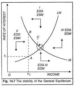
The following diagram (Fig. 14.7) shows that the general equilibrium of the economy which we have derived above is indeed a stable one.

To show this consider all the points to the left of the IS curve, such as point A. At this point, with the given interest rate r₁, the level of income is too low for equilibrium to be achieved in the real sector. This means that expenditure exceeds income and the total value of output is less than the economy’s aggregate demand.

In this situation, producers find their inventories being ran down more than they intend. So they act to increase output. This is the economic force which pushes up national income. For all points to the left of the IS curve, then, there is pressure on income to rise. Similarly, for all points to the right of the IS curve, there is pressure on income to fall.

Now consider points along the LM curve such as points. At this point, with the given level of income Y₁, the interest rate is too high for equilibrium to be achieved in the monetary sector. This means that the supply of real money balances exceeds the demand for real money balances and therefore a downward pressure is exerted on the rate of interest. This is true for all points above the LM curve. It similarly follows that upward pressure will be exerted on the rate of interest at all points below the LM curve.

The directions of the pressure being exerted on incomes and interest rates in the four quadrants of the graph are indicated by the arrows in Figure 14.7. It follows that at any disequilibrium point such as point C, economic forces will be pushing the market towards the general equilibrium position. The actual path to equilibrium may be a spiral, as shown in the diagram rather than a direct route. We can conclude by saying that over a period of time, other things remaining unchanged, stable equilibrium should be reached through adjustments in the goods sector and the money sector.

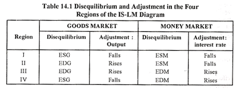
Disequilibrium and Adjustment in the Four Regions of the IS-LM Diagram:

The IS-LM diagram can be divided into four regions starting from I at the north side and going anticlockwise to the second, third and fourth regions situated on the west south, and east. We have already established the equilibrium point at the intersection of the IS curve which slopes down from left to the right and LM curve which slopes up from the left to the right. The IS curve has a negative slope because the real rate of interest must fall in order to equate the increased saving out of rising income with increased investment, as we move from left to right side.

The LM curve has a positive slope showing that as income (output) rises, the demand for money also goes up and the real rate of interest must continue to rise along with income (output) if the equality between the demand for money is to be maintained for a given supply of money. Income (output) and the rate of interest both rise along the LM curve. We can now take up each region and find out the nature of the disequilibrium position which prevails there. We also study the adjustments in output and interest rates induced in each region.

Region I:

Every point in the region I is to the right of the IS curve and to the left of the LM curve. This means that within the region I there is excess supply of goods as well as excess supply of money. Both the level of output (income) and the rate of interest have to fall so that the equilibrium of the economy is reached where the goods sector and the money sector are in equilibrium by themselves and in relation to each other. The arrows indicate the adjustment process.

Region II:

We explain region III because it is the opposite of Region I as far as the nature of disequilibrium is concerned. Every point in this region shows excess demand for goods and also excess demand for money. The excess demand in both the markets forces up expansion of output and rise in the rate of interest at the same time. The arrows drawn in the region show this adjustment process.

Region III:

Every point in this region lies to the left of the IS curve and to also to the left of the LM curve. This shows excess demand for goods because we have to move to the right side in order to reach the IS curve i.e., output expansion is necessary for adjustment. At the same time there is down ward pressure on the rate of interest so that a point on the LM curve can be attained. The downward process on the real rate of interest is due to the excess supply of money at all points in the region II.

Region IV:

The situation in the region IV is the opposite of that in Region II. Every point in this region lies to the right of the IS curve and also to the right of the LM curve. This shows excess of demand both for goods and money in this region. The excess demand must be eliminated through contraction of output and contraction of the demand for money at the same time.

As a result, output must fall and the real rate of interest must rise in order to carry out the adjustment in the two markets of the economy. The arrows point to the directions of the adjustments in output and the interest rate. We have summarised the adjustments in the four regions in Table 14.1.

Shifting of the IS and LM Curves:

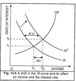
We have demonstrated the stability of the IS-LM equilibrium. We now consider the changes brought about in the economy by shifts in these curves. Let us consider first the effects of an autonomous increase in investment spending.

If equilibrium in the economy is to be maintained, a higher level of saving and therefore national income is required at every interest rate. For this, the A curve has to shift to the right, as shown in the Figure given below. This causes the equilibrium level of income to rise from Y₁ to Y₂ and the equilibrium rate of interest to rise from r₁ to r₂. What is the reason? It is that the higher income level will have brought forth an increased transactions demand for money.

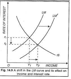
Secondly, let us consider the effect of an autonomous increase in the real money balances. This is the nominal money stock or a fall in the general price level. As a result, the LM curve will shift to the right, as shown in the figure. This happens because every income level (which determines the transactions demand for money) must now be associated with a lower interest rate (and therefore a higher speculative demand for money) if equality between the total demand for and supply of money is to be maintained.

We can find in the diagram that the new equilibrium is associated with a lower rate of interest r₂ and a higher level of income Y₂. In this case, the increased money supply reduces the interest rate which, in turn, causes a rise in the investment spending. It is this rise in investment which pushes up the level of income.