Classical Theory of Income, Output and Employment Determination

The Classical economists disagreed with the Mercantilist view who emphasized State interference and money factors, for the determination of real variables like output and employment.

According to Adam Smith, “it is the real factor which is more important.” Money was used only as a medium of exchange.

Assumptions:

1. Short-Run

2. Full Employment

3. No State Interference

4. Price Mechanism

5. State of Technology and Population is constant

The Classical model of employment consists of 2 components:

I. Aggregate Production Function:

Production function shows the relationship between input and output. Assume there are two inputs—Labour and capital. Due to the assumption of short-run, output will be a function of Labour (N) with capital constant (K), that is, output can be increased only by increasing the variable factor (N) with fixed factor (K) constant.

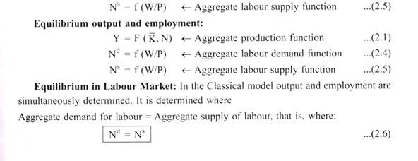
Y = F(K, N) …(2.1)

Where K → Constant capital stock

N → Quantity of homogeneous Labour Input

Y → Real Output.

II. Labour supply and demand function:

With the help of these two functions output and employment is determined. As capital is constant in the short-run, output will change only with change in the labour input.

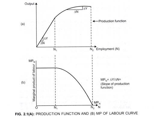
As MP_N represents addition to output when the Labour input is increased, MP_N curve represents the slope of production function.

MP_N = ∆Y/∆N

The slope of the production function (MP_N) is positive but decreases as we move along the curve.

Characteristics of Production Function:

In short run, production function shows technological relationship between the output level (Y) and the level of employment (N).

1. At low level of Labour input before N₁

The Production function is a straight line which exhibits constant returns to scale.

Therefore, MP_N curve is flat which represents constant MP_N.

It shows at very low level of output as we employ more labour to the given capital, productivity of the last worker added does not fall.

Therefore, MP_N does not fall.

2. After N, till N₂

As we add more labour, output increases but at a decreasing rate (i.e., increment to the output decreases) MP_N decreases but is positive.

3. Beyond N₂

The additional Labour employed will not lead to additional production/ output i.e, MP_N = 0.

Therefore, MP_N curve touches X-axis at N₂.

Employment:

The Amount of Labour employed will be determined at the point where:

Aggregate Demand for Labour (N^d) = Aggregate Supply of Labour (N^s)

Assumptions:

1. Market works well.

2. Firms and individual workers optimize.

3. Both the firms and workers have perfect knowledge about the prices.

4. Money wage is adjusted automatically by the market.

5. Perfect competition.

II. (a) Demand for Labour:

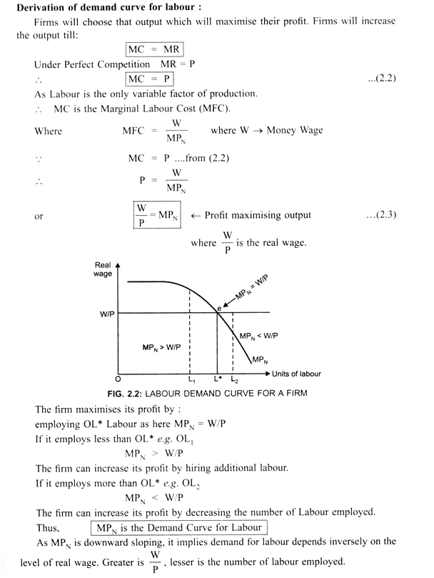
Demand for labour is negatively related to the real wages (W/P). This is because real wages are the cost of production for the firms. Therefore, an increase in real wages due to increase in wages will lead to an increase in the cost of production. This in turn will decrease the profits of the firm because profit is equal to Revenue minus cost (Profit = Revenue – Cost). Due to decrease in the profit level, firm will demand less labour.

Aggregate Demand for Labour (N^d):

It is a horizontal summation of individual firm’s demand curve for Labour. Aggregate demand for labour is negatively related to the real wages (W/P)

N^D = f (W/P) (Aggregate labour demand function) …(2.4)

II. (b) Supply of Labour:

Supply of labour is positively related to the real wages (W/P). This is because wages are the income of the labourer. Increase in wages implies increase in income, therefore, a labourer is willing to work more at higher wages. Thus, the supply curve of labour is positively sloped.

Derivation of supply curve of labour:

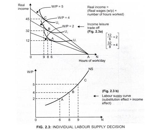
Labour supply curve is derived from the income-leisure trade-off curve which shows the trade-off between leisure and work.

At lower income level, labour prefers work to leisure → Substitution Effect (SE) > Income Effect (IE)

At ‘extremely’ higher income level, labour prefers leisure to work → IE > SE. Thus, we get backward bending supply curve of labour.

However ‘extremely’ high wages are rare. Therefore, it is assumed that the Aggregate labour supply curve has a positive slope. SE is strong enough to offset the IE. (SE > IE)

Individual will supply labour up to the point where:

Slope of income leisure trade off line (shown by the slope of budget line) is equal to the slope of income leisure trade off curve (slope of Indifference Curve).

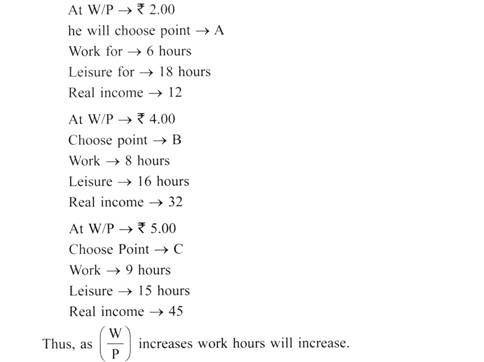
In Fig. (2.3b), by plotting A, B, C at real wages 2.00, 4.00 and 5.00, respectively, we get the labour supply curve which has a positive slope, showing as (W/P) increases more labour is willing to work.

Aggregate Supply Curve of Labour (N^s):

It is a horizontal summation of all individual labour supply curves. It gives the total labour supplied at each level of real wages. It is positively related to the real wages.

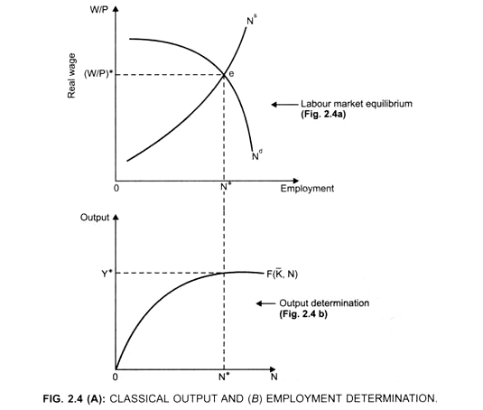
Therefore, Equilibrium level of employment → N*, as here N^d = N^s shown by point ‘e’

Real wage → (W/P)* (Fig. 2.4a)

Equilibrium level of output →Y* (Fig. 2.4b)

Thus, Y* is the full employment level.

Note:

In the classical model →

The endogenous variables are Output, Employment, Real Wage (they are determined within or by the model).

It is the exogenous variable (determined outside the model) which leads to changes in output and employment.

The factors which are operating on the supply side determines the level of output and employment. Thus, it is the supply of labour which plays an important role in the determination of labour market equilibrium and thus the employment and output level.

Conclusion:

Thus, in the classical model the factors that determine the output and employment are the factors which determine the positions of:

(a) Labour supply curve,

(b) Labour demand curve, and

(c) Aggregate Production Function.