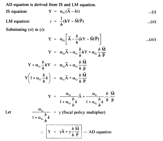
The IS and LM curves together determine the AD schedule. The AD curve maps out the IS-LM equilibrium.
AD curve is drawn on the basis of following assumptions:
1. A Constant.
2. Nominal Money Supply (M) is constant.
ADVERTISEMENTS:
3. Only Price level varies [because AD shows inverse relationship between price and quantity demanded],
AD curve shows the amount of equilibrium output demanded at each price level.
Derivation of AD Equation:
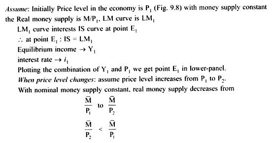
When the price level increases with nominal money supply constant, the real money supply (M/P) will decrease.
ADVERTISEMENTS:
This in turn will lead to an increase in the interest rate which in turn will decrease the investment. As a result the LM curve will shift upwards to the left and AD will decrease.
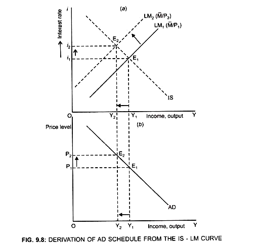
Thus, Y1 corresponds to point E1 on AD curve at point level P1 in the lower panel.
As a result LM curve will shift upwards to the left from LM1 to LM2 and new equilibrium is established at point E2.
ADVERTISEMENTS:
At point E2: IS = LM2
Equilibrium income → Y2 (Y2 < Y1); interest rate rises to i2 (i2> i1)
Y2 corresponds to point E2 on the AD curve at price level P2 and we get point E2 in the lower panel.
Similarly, we can generate many points on the AD curve.
By joining the points E1 and E2, the AD curve is derived which is negatively sloped showing price and output level are inversely related.
This is because:
When P ↑ → real balance (M/P) ↓ → ↑I → ↓ AD → ↓ Y


