In this article we will discuss about Managerial Decision-Making Environment:- 1. Concept of Decision-Making Environment 2. Decision-Making Environment under Uncertainty 3. Risk Analysis 4. Certainty Equivalents.
Concept of Decision-Making Environment:
The starting point of decision theory is the distinction among three different states of nature or decision environments: certainty, risk and uncertainty.
The distinction is drawn on the basis of the degree of knowledge or information possessed by the decision-maker. Certainty can be characterized as a state in which the decision-maker possesses complete and perfect knowledge regarding the impact of all of the available alternatives.
In our day-today conversation, we use the two terms ‘risk’ and ‘uncertainty’ synonymously. Both imply ‘a lack of certainty’. But there is a difference between the two concepts. Risk can be characterized as a state in which the decision-maker has only imperfect knowledge and incomplete information but is still able to assign probability estimates to the possible outcomes of a decision.
ADVERTISEMENTS:
These estimates may be subjective judgments, or they may be derived mathematically from a probability distribution. Uncertainty is a state in which the decision-maker does not have even the information to make subjective probability assessments.
It was Frank Knight who first drew a distinction between risk and uncertainty. Risk is objective but uncertainty is subjective; risk can be measured or quantified but uncertainty cannot be. Modern decision theory is based on this distinction.
In general, two approaches are used to estimate the probabilities of decision outcomes. The first one is deductive and it goes by the name a priori measurement; the second one is based on statistical analysis of data and is called a posteriori.
With the priori method, the decision-maker is able to derive probability estimates without carrying out any real world experiment or analysis. For example, we know that if we toss an unbiased coin, one of two equally likely outcomes (i.e., either head or tail) occur, and the probability of each outcome is predetermined.
ADVERTISEMENTS:
The a posteriori measurement of probability is based on the assumption that past is a true representative (guide to) of the future. For example, insurance companies often examine historical data in order to determine the probability that a typical twenty-five year-old male will die, have an automobile accident, or incur a fire loss.
Thus the implication is that even though they cannot predict the probability that a particular individual will have an accident, they can predict how many individuals in a particular age group are likely to have an accident and then fix their premium levels accordingly.
By contrast, uncertainty implies that the probabilities of various outcomes are unknown and cannot be estimated. It is largely because of these two characteristics that the decision-making in an uncertain environment involves more subjective judgment.
Uncertainty does not seem to suggest that the decision-maker does not have any knowledge. Instead it implies that there is no logical or consistent approach to assignment of probabilities to the possible outcomes.
ADVERTISEMENTS:
Some Characteristics of a Decision Problem:
All business decision problems have certain common characteristics.
These not only constitute a formal description of the problem but also provide the structure necessary for a solution:
1. A decision-maker
2. Alternative courses of action (strategies)
3. Events or outcomes
4. Consequences or payoffs.
In order to illustrate these common characteristics of a decision problem, we may start with a simple real life example. Suppose you are the inventory manager of Calcutta’s New York, which is selling men’s dresses. Your company is not a dress manufacturer. It is just a retail store selling readymade garments. You have to decide how many men’s T-shirts to order for the summer season.
The manufacturer of these has imposed a condition on you: You have to order in batches of 100. If only 100 T-shirts are ordered, the cost is Rs. 10 per shirt, if 200 or more are ordered, the cost is Rs. 9 per shirt; and if 300 or more shirts are ordered the cost is Rs. 8.50.
ADVERTISEMENTS:
The results of market survey provide you with information that the selling price will be Rs. 12 and that the possible sales levels are 100, 150, or 200 units. But you cannot assign any probability estimate to the alternative levels of demand or sales.
If any T- shirt remains unsold during summer, it can be disposed off at half the price in winter. The marketing manager also feels that there is a goodwill loss of 50 paise for each T-shirt that consumers want to purchase from your shop but cannot because of inadequate supplies.
It is not possible for you to wait for some time to study the nature (or determine the level) of demand, nor can you place more than one order. Thus, a situation of complete uncertainty prevails.
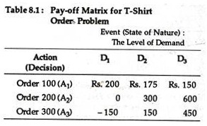
In our example, the decision-maker is the inventory manager, who must decide how many T- shirts to order in the face of uncertain demand. The three alternative strategies are to order 100 shirts (A1), 200 (A2) or 300 (A3).
ADVERTISEMENTS:
The states of nature (which are external to and beyond the control of the inventory manager) are the events and in this case are three levels of demand: 100 (D1), 150 (D2), or 200 (D3). Since the inventory manager does not know which of the events will occur, he is forced to make his decision in the face of uncertain outcomes.
The consequences are measures of the net benefit or payoff (reward) association with each of the levels of demand. The specific consequence or outcome depends not only on the decision (A1, A2, or A3) that is made but also on the event (D1, D2, or D3) that occurs.
That is, there is a consequence or outcome associated with each combination of decision or action and event. These consequences are generally summarized in a payoff matrix.
ADVERTISEMENTS:
The Payoff Matrix:
A payoff matrix is an essential tool of decision-making. It is a nice way of summarizing the interactions of various alternative action and events. Thus we can say that a payoff matrix provides the decision-maker with quantitative measures of the payoff for each possible consequence and for each alternative under consideration.
Positive payoff implies profit and negative pay-off implies loss. For the T-shirts inventory and ordering problem, the payoff matrix is presented in Table 8.1
If the future event that will occur could be predicted with certainty, the decision-maker would merely look down the column and select the optimal decision. If, for instance, it were known for certain that demand would be 150 T-shirts, the decision-maker would order 200, in order to maximize his pay-off.
However, since the decision-maker does not have any knowledge about which event (state of nature) will occur or what is the chance of a particular event occurring, he is faced with a situation of total uncertainty.
Decision-Making Environment under Uncertainty:
ADVERTISEMENTS:
We may now utilize that pay-off matrix to investigate the nature and effectiveness of various criteria of decision making under uncertainty.
Four major criteria that are based entirely on the payoff matrix approach are:
(1) Maximin (Wald),
(2) Maximax,
(3) Hurwicz alpha index, and
(4) Minimax regret (Savage).
ADVERTISEMENTS:
In those situations where the decision-maker is willing to assign subjective probabilities to the possible outcomes, the two other criteria are
a. The Laplace (Bayes’) and
b. The maximization of expected value.
It may be noted that once subjective probabilities are introduced, the distinction between risk and uncertainty gets blurred.
1. Maximin:
The maximin (or Wald) criterion is often called the criterion of pessimism. It is based on the belief that nature is unkind and that the decision-maker therefore should determine the worst possible outcome for each of the actions and select the one yielding the best of the worst (maximin) results. That is, the decision-maker should choose the best of the worst.
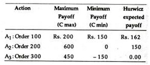
In our T-shirt example the minimum payoffs associated with each of the actions are presented below:
If the decision-maker is a pessimist and assumes that nature will always be niggardly and uncharitable the optimal decision would be to order 100 T- shirts because this action maximizes the minimum payoff. Thus, the criterion is conservative in nature and is well-suited to firms whose very survival is at stake because of losses.
2. Maximax:
An exactly opposite criterion is the maximax criterion. It is known as the criterion of optimism because it is based on the assumption that nature is benevolent (kind). Thus, this criterion is suitable to those who are particularly venturesome (extreme risk takers).
In direct contrast to the maximin criterion the maximax implies selection of the alternative that is the “best of the best”. This is equivalent to assuming with extreme optimism that the best possible outcome will always occur.
In our example, the best possible outcome, given each of the levels of demand, are the following:
The decision-maker would thus choose to order 200 units because this offers the maximum possible payoff.
3. Hurwicz Alpha Index:
ADVERTISEMENTS:
The Hurwicz alpha criterion seeks to achieve a pragmatic compromise between the two extreme criteria presented above. The focus is on an index which is based on the derivation of a coefficient known as the coefficient of optimism.
Here the decision-maker considers both the maximum and the minimum payoffs from each action and weighs these extreme outcomes in accordance with subjective evaluations of either optimism or pessimism.
If, for instance, we assume that the decision-maker has a coefficient of 0.25 for a particular set of actions, the implication is clear. He has implicitly assigned a probability of occurrence of 0.25 to the maximum payoff and of 0.75 to the minimum payoff.
As a general rule the value of following a particular action can be determined according to the following index:
Hi =αCmax + (1 – α)Cmin (8.1)
The decision-maker would then pick that option which yielded the maximum Hi value. Equation (8.1) indicates that the more optimistic the decision maker, the larger will be the Hi value, and vice versa. A value of alpha (a) equal to 0.5 implies that the decision-maker is neither an optimist nor a pessimist.
The results of applying the Hurwicz criterion in Eq. (8.1) assuming an alpha value of 0.25 are presented below:
Thus, the decision-maker would choose A1, i.e., order 100 T-shirts. The major drawback of this decision criterion, however, is the assignment of probabilities for the states of optimism and pessimism.
4. Minimax Regret:
The minimax regret has been proposed by Savage. This criterion suggests that after a decision has been made and the outcome has been noted, the decision-maker may experience regret because by now he knows what event occurred and possibly wishes that he had selected a better alternative. Thus, this criterion suggests that the decision-maker should attempt to minimize his maximum regret.
The implication is that the decision-maker would develop a regret (opportunity loss) matrix and then apply the minimax rule to select an action. Regret is defined as the difference between the actual payoff and the expected pay-off, i.e., the payoff that would have been received if the decision maker had known what event was going to occur.
The conversion of a payoff matrix to a regret matrix is very easy. All we have to do is to subtract each entry in the payoff matrix from the largest entry in its column.
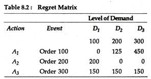
It is quite obvious that the largest entry in every column will have zero regret. The implication is that if the decision-maker had indeed selected that action, he would have experienced no regret (that is, no opportunity loss). Table 8.2 depicts the regret matrix for the T-shirt inventory problem.
The regret value in Table 8.2 represent the difference in value between what one obtains for a given action and a given event and what one could obtain if one knew beforehand that the given event was, in fact, the actual event. For example, if 100 T-shirts are ordered and demand is 150 units, then regret is Rs. 125, as Rs. 300 (Rs. 125 more) could be received by ordering 200 units.
Thus, if the decision-maker had known that demand was going to be 150 T-shirts, his optimal decision would have been to order 200 T-shirts; if he had ordered only 100 T- shirts his opportunity loss would be Rs. 125. The remaining entries in the regret matrix are computed by following the same procedure, i.e., by comparing the optimal decision with the other possibilities.
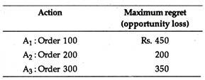
The maximum regret values for each of the action or actions are presented below:
The smallest possible regret (or minimum opportunity loss) would be incurred by ordering 200 units. If the original payoff table is stated in terms of losses or costs, the decision-maker will then select the smallest loss for each event and subtract this value from each row entry.
a. Laplace (Bayes’) Criterion:
The Laplace criterion of insufficient reason differs from the minimax regret criterion in that it involves the use of probabilities, that is, if we are uncertain as to which event will occur, we can assume (correctly or incorrectly) that all states (levels of demand) are equally likely and then assign the same probability to each of the events, i.e., we assume that each event is equi-probable.
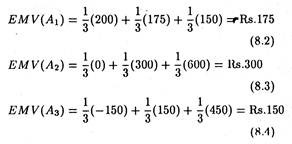
These probability assignments can then be utilized to calculate the expected payoff for each action and to choose that action with the maximum (smallest) expected payoff (loss). For the T-shirt example, the probability assigned to each of the three events would be 0.33, and the expected monetary value (EMV) would be
Therefore, following the Laplace criterion, the decision-maker would order 200 units because it has the highest expected value. This criterion is, however, criticized on the ground that the assumption of equally likely events may be incorrect and the user of this criterion must consider the basic validity of the assumption.
b. Maximizing Expected Value:
This criterion is also based on the assignment of probabilities. However, the assumption that each event is equi-probable is not made. Instead, the analyst makes a more critical appraisal before assigning subjective probabilities to each event. By assigning subjective probabilities, the decision maker is, in essence, converting an uncertain situation into a situation of risk.
Suppose, for example, the inventory manager and the marketing manager reach a consensus of opinion that the applicable probabilities for these different states of nature are: sell 100 units, 0.5; sell 150 units, 0.3; and sell 200 units, 0.2. Since the events are mutually exclusive, the sum of their probabilities is equal to 1.
Based on this estimation of probabilities, the expected payoff can be computed as follows:
A1 (100) = 0.5 (Rs. 200) + 0.3 (Rs. 175) + 0.2 (Rs. 150) (8.5)
= Rs. 182.50
A2 (200) = 0.5 (0) + 0.3 (Rs. 300) + 0.2 (Rs. 600) (8.6)
= Rs. 210.00
A3 (100) = 0.5 (Rs. 150) + 0.3 (Rs. 150) + 0.2 (Rs. 450) (8.7)
= Rs. 60.00
Therefore, by using the maximization of expected value criterion, the inventory manager would choose A2, i.e., order 200 units.
A useful extension of the expected value criterion is the expected opportunity loss (EOL) criterion. It differs from the EMV in the sense that it involves the use of the regret matrix.
In our example, the expected opportunity losses can be computed as:
EOL (A1) = 0.5(0) + 0.3 (Rs. 125) + 0.2 (Rs. 450) (8.8)
= Rs. 127.50
EOL (A2) = 0.5 (Rs. 200) + 0.3 (0) + 0.2 (0) (8.9)
= Rs. 100.00
EOL (A3) = 0.5 (Rs. 350) + 0.3(Rs. 150) + 0.2(Rs. 150) (8.10)
= Rs. 250.00
The EOL criterion leads us to take the minimum EOL, which, in the T-shirt example, would be to order 200 units.
Summary:
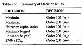
The results of employing the six criteria to our T-shirt example are given in Table 8.3. It is clear that there is no perfect convergence of decisions, although A2 is dominant. In the final analysis, the inventory manager can easily toss out the A3 option, but he must still bear the burden of choosing A1 or A2 in the face of uncertain demand.
Expected Value of Perfect Information (EVPI):
So long our stress was on selection of an alternative on the basis of information currently possessed by the decision-maker. In most real-life situations, the decision-maker has the option of gathering additional information before arriving at a decision.
To a rational decision-maker, the value of information can be treated as the difference between what the payoff would be with the information currently available and the payoff that would be earned if he were to know with certainty the outcome prior to arriving at a decision.
Simply put, the value of perfect information is the difference between the maximum profit in a certain environment and the maximum profit in an uncertain environment.
In our T-shirt example, the EMV under conditions of uncertainty for the optimal decision of ordering 200 units was found to be Rs. 210. To compute the EMV under conditions of certainty, we start with the assumption that the decision-maker selected the option with the highest payoff for each of the alternatives.
For example, if the inventory manager knew, before arriving at the decision, that actual demand were going to be 100 units, the optimal decision would be to order 100 units with a payoff of Rs. 200; if demand were going to be 150 units, he would place order for 200 units with a payoff of Rs. 300 and if demand were 200 units, he would order 200 and the payoff would be Rs. 600.
To compute the expected value of perfect information, we simply apply the same probabilities that were used in the EMV computations to these certain payoffs:
Expected profit under certainty
= 0.5 (Rs. 200) + 0.3 (Rs. 300) + 0.2 (Rs. 600)
= Rs. 310 (8.11)
Therefore, in our example, the expected value of perfect information is to be computed as follows:
EMV under conditions of certainty = Rs. 310
EMV under conditions of uncertainty = Rs. 210
Expected value of perfect information = Rs. 100
Thus, the inventory manager knows that the maximum amount that he would pay for a perfect prediction of demand would be Rs. 100. To pay more for perfect information than the loss that would result because of a lack of this information (uncertainty) would be irrational.
However, it is virtually impossible, in practice, to gather perfect information. Yet the computation of its value is extremely useful to a manager. For example, if he believes that the probability that additional information will be correct is 0.3, the value of this information would be Rs. 30 (Rs. 100 x 0.3).
The basic point to note here is that they provide the decision-maker with a procedure for evaluating the benefits of obtaining additional information and comparing them with the costs of this information.
Sensitivity Analysis:
One major drawback in the use of the EMV, EOL or EVPI is the method used to assign probabilities to the events. In particular, managers are likely to say “I feel the probability of this event occurring is between 0.3 and 0.5”. Under these circumstances sensitivity analysis often bears fruit because it provides a measure of how probability assignment affects the decision.
Suppose, our inventory manager had obtained a different set of probability estimates for the three levels of T-shirt demand — that is, the probabilities are 0.2 for 100, 0.3 for 150 and 0.5 for 200 T- shirts. Based on these probabilities the expected value of the three actions (order 100, 200 or 300) would be Rs. 167.50, Rs. 390 and Rs. 240, respectively.
The optimal decision would still be the same, viz., ordering 200 units; thus the manager’s decision is not very much sensitive to changes in the probability assignments. This assumes strategic significance both in reducing the anxiety surrounding the decision and in measuring the need for additional information.
Additional Examples:
Example 1
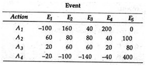
Suppose that you have the following payoff matrix:
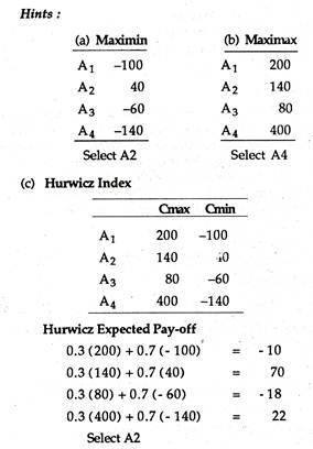
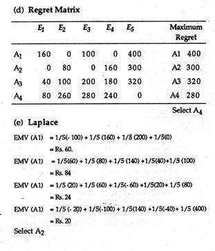
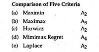
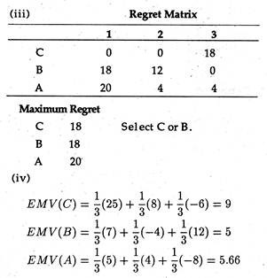
Select the optimal action by applying maximin, maximax, Hurwicz (= 0.3 ), minimax regret and the
Laplace criteria. Compare your choice under each criteria.
Example 2:
A marketing manager has to determine in which of two regions a new product should be introduced. The level of sales can be characterized as either high, average or low. He estimates that the probabilities associated with each of these outcomes are 0.25, 0.50 and 0.25, respectively.
The payoff matrix has been constructed as follows:
Using EMV as a criterion, in which of the two regions should the product be introduced?
Solution:
EMV(A1) = 0.25 (40,000) + 0.50 (30,000)+ 0.25 (20,000)
= Rs. 30,000
EMV (A2) = 0.25 (70,000) + 0.50 (20,000) + 0.25 (0)
= Rs. 27,500
Select A1
Example 3:
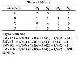
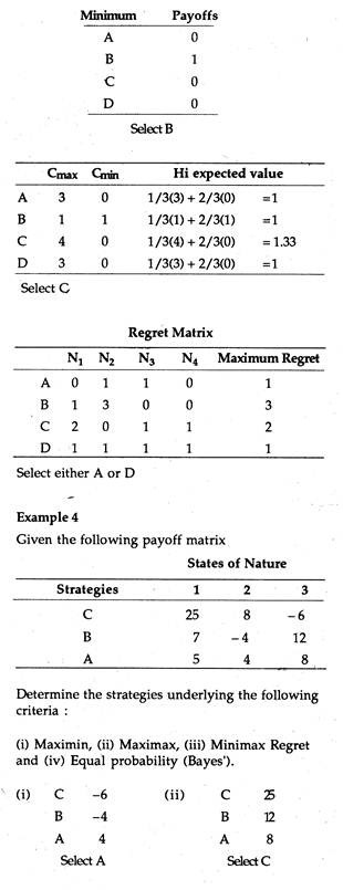
In the following payoff matrix of a decision problem show that strategy A will be chosen by the Bayes’ criterion, strategy B by the maximin criterion, C by the Hurwicz α (for α < 1/2) and D by the minimax regret criterion:
Example 5
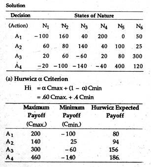
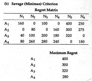
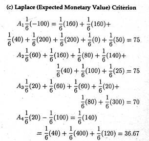
Consider a hypothetical 4 x 6 payoff matrix representing a maximizing problem of decision-maker, faced with total uncertainty. Find out his optimal strategy considering that (a) he is a partial optimist (Hurwicz criterion, with the coefficient of optimism 60%), (b) he is an extreme pessimist (Savage criterion) and (c) he is a subjectivist (Laplace criterion).
Since it has the highest payoff the decision-maker would choose A4.
If the minimax criterion is followed, the decision maker would again choose A4.
Since the first decision (A1) has the highest expected value it will be taken.
Decision-Making Environment under Risk Analysis:
Here we drew a distinction between risk and uncertainty. Recall that risk is characterized as a state in which the decision-maker has only imperfect information about the decision environment, i.e., the impact of all of the available alternatives. But the decision-maker is still able to assign probability estimates to the possible outcomes of a decision.
These estimates are either subjective judgments or may be derived from a theoretical probability distribution. Uncertainty refers to a state in which the decision-maker lacks even the information to assign subjective probabilities.
This distinction was first drawn by F. H. Knight who noted that risk is objective but uncertainty is subjective. Yet, the two terms are often used interchangeably to mean simply ‘a lack of certainty’.
However, the important point to note is that the use of subjective probabilities has diminished the significance of the distinction between risk and uncertainty. In other words, by assigning subjective probabilities to decision problems, decision-making under uncertainty can easily be converted into risk analysis.
i. Treatment of Risk in Economic Analysis:
Risk analysis involves a situation in which the probabilities associated with each of the payoffs are known.
There are two alternative ways of deriving these probabilities:
(a) By an analysis of historical patterns, or
(b) By reference to a theoretical probability distribution (such as the binomial distribution, Poisson distribution or normal distribution).
Risk analysis is based on the concept of random variable. A random variable is any variable whose value is uncertain, that is, whose value is subject to probabilistic variation.
For example, when one rolls a die the number that comes up is a random variable. The price of tea next week may also be random owing to unforeseen shifts in supply and demand. Now the values that a random variable can assume may not be equally likely (i.e., equi-probable events).
For this reason it is necessary to look at the probability distribution of the random variable, which is a listing- of the possible outcomes with the associated probabilities of those outcomes.
For the roll of a die, the probability distribution is as follows:
Here we let X denote the number on the face of the die and P(X) represents the probability of that outcome. In this case, the six possible outcomes are equally likely (i.e., each one is an equi-probable event.)
Expected Value:
An important characteristic of a random variable is its expected value or mean. Recall that the expected value is a weighted average of the possible outcomes, where the weights are the objective probabilities of possible outcomes.
The expected value (denoted by E) of the outcome when a fair die is rolled is:
The primary decision criterion in an environment characterized by risk is the expected value (E) criterion.
The criterion can simply be stated as:
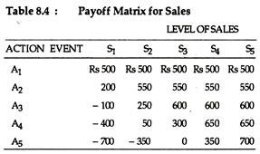
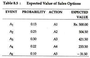
where the Xs refer to the payoffs from each event and to the probabilities associated with each of the payoffs. The concept may now be illustrated. Suppose we have the following pay-off matrix (Table 8.4). Table 8.5 lists the respective probabilities for each of the events and the associated expected values.
If the decision-maker analyses the expected values of each of the actions, he arrives at the decision to select the option which is having the highest expected value, i.e., option 2 in this example.
However, the difficulty with the expected value criterion is that on the basis of it, one cannot always make an unambiguous decision. If, for instance, the probabilities or the pay-offs were changed such that A2 and A3 had the same expected value of Rs. 504.50, it would be difficult for the decision-maker to measure the degree of risk associated with each action and thus arrive at a clear- cut decision. In such a situation some criterion has to be tried to arrive at a relative measure of risk.
ii. Measurement of Risk:
The expected monetary value (EMV) criterion no doubt furnishes necessary and useful information to the decision-maker. But its major defect is that it can obscure the presence of abnormally high potential losses or exceptionally attractive potential gains. True, expected value is a mathematical average the mean of a probability distribution that neatly summarizes an entire distribution of outcomes.
This simply explains why a decision maker who passes decisions solely on expected value is likely to make choices that are inconsistent with his psychological preferences for risk taking. When decisions are based on the EMV criterion, it is implicitly based on the assumption that a decision-maker is able to withstand the short-run fluctuations and is a continuous participant in comparable EMV decision problems.
For their own survival, however, decision-makers commonly choose a course of action that is supposed to provide a satisfactory return subject to the acceptance of a certain degree (level) of risk.
With our present state of knowledge, the most useful way of measuring the degree of risk from the perspective of a decision-maker, is the nature of the probability distribution — more specifically, its spread or dispersion about a mean.
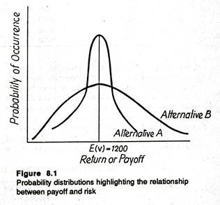
In truth, the less dispersed the probability distribution of possible outcomes, the smaller the degree of risk of any given decision. In other words, the closer the values of all possible outcomes are to the expected value, the less risky the choice is likely to be. Fig. 8.1 illustrates this observation.
Here, for the sake of simplicity, we consider only two probability distributions. Each alternative gives the same payoff or EMV of Rs. 1200.
However, the distribution of possible outcomes is more closely concentrated around this expected payoff for alternative A than it is for alternative B, i.e., for B it is more spread out around E(V). So according to our criterion, alternative A would be treated as less risky than alternative B.
Thus even if the two alternative have the same EMV, the decision maker would choose the option having the least dispersion (or maximum concentration). Students with some background of statistics know that the simplest measure of dispersion of the possible outcomes around the mean (i.e., expected value) is the standard deviation of the probability distribution.
It is expressed as:
We illustrate the concept in table 8.6 below:
If we adopt the simple EMV criterion, a cursory glance would make project B apparently seem to be the best possible choice. However, a closer scrutiny of the cash flows also reveals that project A has a small expected value, but, at the same time, it shows less variation and according to our yardstick, appears to be less risky.
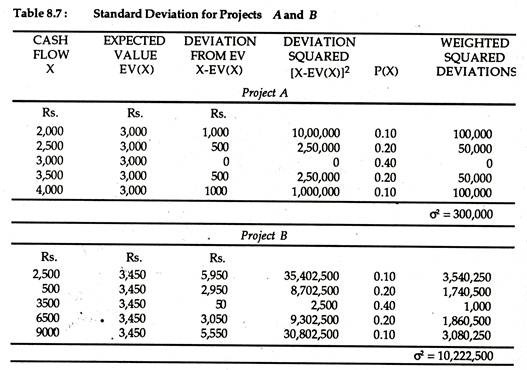
By putting the values of cash flow (X), expected value (EMV), and assigned probability from Table 8.6 into equation (8.13) we are in a position to quantify this risk. The results of our calculations are shown in Table 8.7.
We simply calculate the standard deviation for project A and B as the square root of the variances σA2 and σB2. Thus we get σA = Rs. 547.7 for project A and σB = Rs. 3197.3 for project B. Thus, the project B has a higher EMV but it is risker since it has a higher standard deviation. In other words, even if the returns from project B are higher on average than that of A, the former exhibits greater variability. Hence, it involves more risk.
If, however, two projects or alternatives have significantly different expected monetary values, we can use standard deviation to measure relative risk of the two projects. Suppose, that project A has an EMV of Rs. 500,000 and a standard deviation of Rs. 500, whereas project B has an EMV of Rs. 100,000 and a S.D. of only Rs. 200.
In such a situation, we cannot compare the two projects so easily by using the standard deviation measure. Here a new measure of relative risk, known as the coefficient of variation or the index of relative risk, is often used.
This is expressed as:
In case of two or more projects (alternatives) having unequal costs or benefits (payoffs) the CV is undoubtedly a preferable measure of relative risk. In our example, the coefficients of variation for projects A and B are, respectively, 0.001 and 0.002.
Thus, according to our criterion, project A is less risky than project b. From Table 8.7 we can compute CV for project A and B. For project A it is 0.183 and for project B, 0.297. This simply indicates that project b is characterized by greater degree of risk than project A.
Subjective Probability:
So long we restricted ourselves to considerations of risk involving objective probabilities. Such objective probability is couched in terms of relative frequency. In fact, the probability of an event’s happening is the relative frequency of its occurrence. This concept of probability is said to be objective in the sense that the values can be determined experimentally as in tossing a coin 10 times, or rolling a fair die 100 times.
In some cases, however, a relative frequency (also known as the classical) interpretation of probability does not work because repeated trials are not possible. One may, for instance, ask what is the probability of successfully introducing a new breakfast food (like Maggie).
Since there are constant changes in market conditions and in the number (range) of competitive (rival) products, it is not possible to repeat the experiment under the same conditions hundreds of times. In such situations the decision-maker has to assign probabilities on the basis of his own belief in the likelihood of a future event. These probabilities are called subjective probabilities.
The decision-maker thus attaches his best estimate of the ‘true’ probability to each possible outcome. In reaching decisions he makes use of these subjective probabilities in precisely the same way the objective (or relative frequency) probabilities would be used if they were available.
iii. Profit Planning under Risk and Uncertainty:
In traditional economic theory it is assumed that the firm’s objective is to maximise its profits under conditions of certainty. However, the real commercial world is characterized by uncertainty.
The presence of uncertainty upsets the profit- maximization objective. Let us consider a simple competitive market where the demand (average revenue curve) faced by a seller is a horizontal straight line. The implication is that the firm is a price-maker. It can sell as much as it likes at the prevailing market price. Now let us relax the assumption.
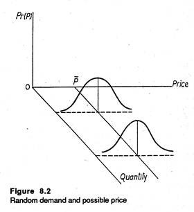
Suppose the horizontal demand curve facing a competitive firm moves up and down in a random (unsystematic) fashion. The implication is that the price that the firm faces is not stable. Rather it is a random variable. In Fig. 8.2 we show the likelihood of a particular price on a given day by the height of the bell-shaped curve.
The fact that the curve is highest for prices very close to the average or expected price P indicates that these prices are most likely. Contrarily, abnormally high or exceptionally low prices are possible but unlikely.
Fig. 8.2 makes one thing clear at least: when demand is random, the actual price is subject to a probability distribution. On average, the price will be equal to the mean price of P. Since price is random, profit will be random, too.
As another example, let us consider the following discrete probability distribution of prices.
It is not possible to know in advance the actual price for tomorrow. But we can calculate the expected price which is
P = 5(0.08)-t 6(0.14) + 7(0.18) + 8(0.20) + 9(0.18) + 10(0.12) + 11(0.08) + 12(0.02)
= Rs. 8.04
This is the average price which is arrived at by multiplying each possible price by the probability of its occurrence and adding up the results.
Random Profit:
Now we have a random price for the firm’s output. It is further assumed that the manager must specify the quantity of output before he observes the actual price that consumers will pay for the commodity. Such things often happen in reality and managers have to face such uncertain situations. For example, farmers face considerable uncertainty about the price they will receive in October for a crop planted in July.
Similarly, producers of new fashion garments and new model wrist watches must often produce a considerable quantity before they are able to know consumers’ reaction to their products. For simplicity, we assume that the product is perishable. So the manager has to sell all the output rather than store some of it for future sales.
Since profit is total revenue (= price x quantity) less total cost of producing the required quantity, profit is also a function of the random price. Consequently, profit is also random.
Since profit is a random variable, the concept of maximum profit becomes meaningless. It is because one cannot maximize something which one cannot control. If profit maximization does not appear to be a sensible goal, one has to search out or identify another objective function for the firm.
Such a new objective function has to take account of two factors:
(1) The firm’s attitude toward risk and
(2) The manager’s perceptions of the likelihood of various outcomes.
It is gratifying to note that the expected utility approach to decision problems under risk accommodates both factors and provides a logical way to arrive at decisions.
iv. Expected Utility Theory and Risk Aversion:
In the context of decision problems whose uncertain possible outcomes constitute rupee payments with known probabilities of occurrence, it has been observed by many that a simple preference for higher rupee amounts is not sufficient to explain the choices (that is, decisions) made by various individuals.
The classic example, known as the St. Petersburg Paradox, and formulated by the famous mathematician, Daniel Bernoulli, about 250 years ago, illustrates a dilemma. Bernoulli observed that gamblers did not respond to the expected rupee prices in games of chances. Instead, he suggested that they responded to the utility that the prizes might produce.
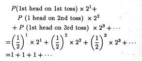
The paradox consists of an unbiased coin (i.e., a coin in which the probability of head or tail is 1/2) which is tossed repeatedly until the first head appears. The player is supposed to receive or win 2n rupees as soon as the first head appears on the n-th toss.
Now the relevant question here is: how much should the player be ready to pay to take part in this gamble (i.e., how much should he be willing to wager)? To answer this question we have to find out the EMV of such a gamble which is:
Here EMV is the sum of an infinite arithmetic series of 1’s.
Thus if we go by the EMV criterion we can assert that the gambler (player in our example) will be ready to wager everything he owns in return for the chance to receive 2n rupees.
However, in real life most people prefer to play safe and avoid risk. Therefore they would decide not to participate in this type of gamble characterized by highly uncertain outcome against an unlimited payment (that has to be made if the gamble is accepted).
Thus, the prediction is that actual monetary values of the possible outcomes of the gamble fail to reflect the true preference of a representative individual for these outcomes. So the maximization of EMV criterion is not a reliable guide in predicting the strategic action or strategic choice of an individual in a given decision environment.
The same conclusion is also reached from other examples of behaviour, such as diversification of investment portfolio as also the simultaneous purchases of lottery tickets (that is gambling) and insurance.
By rejecting maximization of EMV criterion as a valid guide for decision-making in situations involving risk, Von Neuman and Oskar Morgenstern developed an alternative framework (based on expected utilities of the outcomes) which can be utilized for decision-making in a situation of risk.
They have proved conclusively that the Maximization of expected utility criterion, which is a preferable alternative to EMV criterion, yields decisions that are in accord with the true preference of the individual (the player) provided one condition is satisfied: he is able to assess a consistent set of utilities over the possible outcomes in the problem.
They calculate expected utility in the same way expected value is calculated by multiplying the utility of each outcome by its probability of occurrence, and then summing up the whole thing, thus:
This criterion apparently appears to be very effective. But a number of difficulties crop up when we try to implement it. Firstly, in a large organization, whose utility function has to be used remains an open question. Secondly, in case of large private firms characterized by separation of ownership from management whose utility function — the managers’ or shareholders’ — has to be used is another question.
Suppose we decide to use the utility functions of shareholders. Since different shareholders are involved and they have different utility functions, which are not directly comparable, it is virtually impossible to arrive at a group utility function.
Secondly, complex problems arise in measuring the utility function of an individual. Yet with the present state of knowledge, the utility function is the only tool available for incorporating the decision maker’s true preferences for the outcomes of the problem into the decision-making framework.
Illustration:
We may now see how to utilize the new criterion, i.e., the maximization of expected utility criterion in arriving at decisions under risk. Suppose an entrepreneur has developed a new product which is yet to be put into the market. He is considering whether or not to make long-term investment for introducing the product in the market.
Suppose on the basis of intensive market survey and research it is discovered that 20% of such product met with success in the past and the remainder (80%) were failures. It is estimated that the cost of producing and marketing a batch of the product will be Rs. 4,000.
If we assume that a sub-contractor can be engaged to manufacture the product, there is no need for any investment in production facilities. It is also estimated that if the marketing effort is successful, a profit of Rs. 16,000 will result.
We additionally assume that it is very easy to copy the product. Therefore, sooner or later, intensive competition will restrict the profitable sales of the product. Thus the initial amount which is produced can be profitably sold.
On the contrary, if the product is not initially successful and there is total failure of the marketing effort, the maximum amount of loss the entrepreneur has to incur will be Rs. 4,000, i.e., the cost of production and marketing.
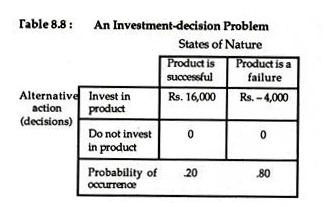
We may now summarize the basic characteristics of the decision problem in the following payoff matrix.
It is quite obvious that the action or decision — ‘Do not invest in the product’ — results in a zero return or pay-off regardless of the decision- environment, i.e., the state of nature. In the row below the matrix we show the probability of occurrence of each state of nature.
The EMV of the decision to ‘invest in the product’ is:
EMV1 = Rs. 16,000 x .20 + (Rs. -4000) x .80 = Re. 0.
On the contrary, for the alternative decision ‘do not invest’ it is:
EMV2 = 0 x .20 + 0 x .80 = Re. 0.
Thus, in this simple example, it is very difficult for the entrepreneur to arrive at a decision on the basis of EMV criterion. Since EMV is the same under two alternative actions the decision-maker would remain indifferent between them.
Now we may incorporate the utility function of the entrepreneur into the decision-making framework and see if it enables the entrepreneur to express his risk preference. His risk reference can be measured by the nature of his utility function.
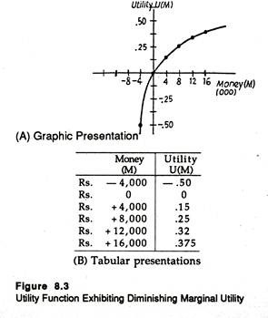
Suppose, in the first case, that the entrepreneur has the utility function, shown in Fig. 8.3.
The utility function is characterized by diminishing marginal utility of money. Recall that the word ‘margin’ always refers to anything extra. Therefore, marginal utility measures the satisfaction the individual receives from a small increase in his stock of wealth.
Here we use the three terms ‘wealth’, ‘money’ and ‘return’ synonymously. The slope of the utility function at any point measures marginal utility.
In reality we observe that as an individual’s stock of wealth (money) increases, every additional unit of wealth gives him gradually less and less extra satisfaction (utility). From this emerges the diminishing marginal utility hypothesis. Here, in Fig. 8.3 the slope of the utility function falls as the decision-maker’s stock of wealth increases. This corroborates the diminishing marginal utility hypothesis.
The implication is simple: as his wealth increases, the individual receives less and less extra utility (satisfaction) from each extra rupee that he receives. Now by using equation (15) we can calculate expected utility, based on the utility function of Fig. 8.3.
For the decision to ‘invest in the product’ it is:
E(U1) = U(Rs. 16,000) x .20 + U(Rs. -4000) x .80
= .375 x .20 + (-.50) x .80
= – .325
For the alternative action, i.e., for the decision ‘Do not invest’ it is:
E(U2) = U(0) x .20 (0) x .80
= 0 x .20 + 0 x .80 = 0
Thus the decision ‘Do not invest’ has a higher expected utility. Therefore, by using the maximization of expected utility criterion, the rational entrepreneur would decide against the project. He would decide not to invest in the new product. Thus diminishing marginal utility of money leads directly to risk aversion. In term of EMV this investment is an example of fair gamble since its EMV is zero.
On the basis of differences in attitude toward risk, decision-makers are classified into three categories: risk-averter, risk-indifferent and risk- lover. In our example the investor is a risk-averter.
A risk-averter is one who, because of diminishing marginal utility of money, expresses a definite preference for not undertaking a fair investment or fair gamble, such as the one illustrated above. It is also possible for the risk-averter to be reluctant to undertake investments having positive EMVs.
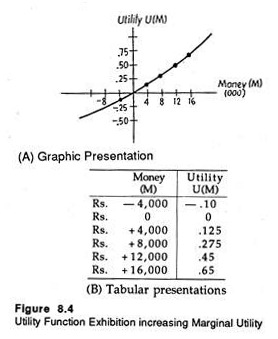
Now let us consider a second situation — an exactly opposite one where the entrepreneur has the utility function, characterized by increasing marginal utility of money. Here the slope of the utility function is increasing as the individual’s wealth increases.
This reveals the increasing marginal utility hypothesis The implication of this hypothesis is simple enough: as the individual’s wealth increases, he receives more extra utility from each extra rupee that he receives.
On the basis of the data which accompany the utility function of Fig. 8.4, the expected utility of the decision to ‘Invest in the Product’ is:
E(U1) = U(Rs. 16,000) x .20 + U(Rs. – 4,000) x .80
= .65 x .20 + (- .10) x .80 = 0.5
It is zero for the alternative action. ‘Do not Invest’, i.e., E(U2) = 0. (Try to guess why.) Thus the optimal decision would be to accept the project, i.e., invest in the product.
A decision-maker who, because of an increasing marginal utility of money, exhibits a definite preference for undertaking actuarially fair investments such as this one is called a risk-lover. It is because he loves to take risk. It is also possible for a risk- lover to be eager and willing to undertake investments having negative EMVs.
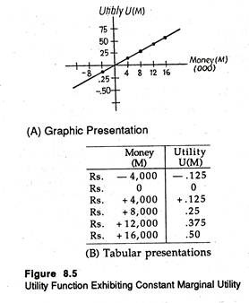
Finally, let us consider a situation in which the entrepreneur has a linear utility function, as shown in Fig. 8.5.
Here the utility function shows constant marginal utility of money. The implication is that as the individual’s wealth increases he receives the same extra utility from each additional rupee that he receives. It is left as an exercise to the reader to demonstrate that the expected utilities of both the decisions: ‘investment in the product’ and ‘do not invest’ are zero.
Therefore, the entrepreneur with a linear utility function would show indifference to the two alternative actions when attempting to maximise expected utility. He would, therefore, be called a risk-indifferent (neutral) decision-maker. It is interesting to note that this is the same decision (that is, indifference) as was obtained in the first part with the EMV criterion.
It is also possible to show that for a risk- neutral individual, the maximization of EMV criterion will generally yield the same decisions as the maximization of expected utility criterion.
The implication of this statement for decision-making purposes is that if the decision-maker feels that he is having a linear utility function over the range of outcomes in a decision problem, there is hardly any need to go through the whole complex process of seeking to derive his utility function of money.
In such a situation, taking the action with the highest EMV will surely lead to decisions that are quite in accord with the true preferences of the decision-maker.
In short, the decision-maker’s attitude toward risk determines the shape of his utility function and assists the choice of alternative in a decision problem involving risk.
v. Sequential Decision Making: Decision Tree Analysis:
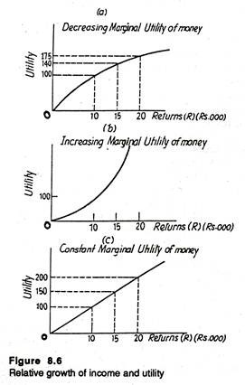
A new technique of decision making under risk consists of using tree diagrams or decision trees. A decision tree is used for sequential decision-making. Suppose Mr. X is a decision-maker with a utility function shown in Fig. 8.6 who has an income of Rs. 15,000, and he is given the following offer.
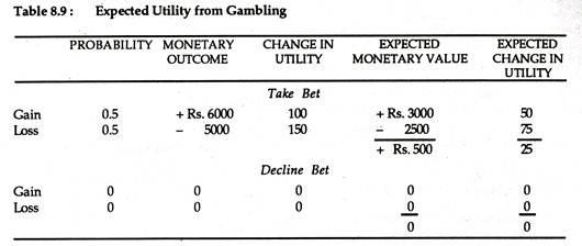
Mr. X’s friend Mr. Y will flip a coin. If a head appears in the first toss Mr. X owes Mr. Y Rs. 5,000; if a tail appears, Mr. Y will pay Mr. X Rs. 6,000. Mr. X’s EMV from playing this gamble is Rs. 500 (a 50% chance of losing Rs. 5,000 supported by a 50% chance of winning Rs. 6,000).
It is worthwhile for Mr. X to decline the bet if the reduction in utility from losing Rs. 5,000 is greater than the increase in utility from winning Rs. 6,000. Table 8.9 and Fig. 8.6 summaries mathematically Mr. X’s decision, i.e., not to take the coin flipping bet, in two different ways.
In Table 8.6, a comparison of the EMV of ‘Take Bet’ with ‘Decline Bet’, shows that the Rs. 500 expected gain from taking the bet is surely better than the zero rupee gain from declining the bet. If we bring into focus the concept of utility, the expected utility loss of 25 from betting is obviously inferior to the no-change outcome.
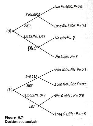
Fig. 8.7 presents the same information using decision trees.
The tree in panel (a) considers monetary gain and loss; the tree in panel (b) shows utility gain and loss. The initial branch of both the trees — upper and lower, represents bet or decline bet decision, with each subsequent branch representing the possible outcomes and the associated probabilities.
After setting forth the probabilities, we calculate the expected monetary values — which are shown in the brackets. We can now compare the figures in brackets — (Rs. 500) and (Re. 0) — in the upper tree with the expected utility figures — (-0.25) and (0) — in the lower tree.
The major advantage of the decision tree approach is its brevity. In fact, it is easier to comprehend ‘trees’ easily than tables when we move to more realistic business situations involving various decisions (branches). Moreover, decision trees highlight the sequential nature of decision-making.
Example:
Choosing a Technique of Production:
Suppose Mr. Ram is a project manager and has been entrusted with the responsibility of developing a new circuit board which is an important component of a colour TV.
The budgetary limit of the project has been set at Rs. 400,000 and Mr. Ram has been given six months time to complete the project. The R&D engineers have succeeded in identifying two approaches, one utilizing conventional materials and another using a newly developed chip.
It has been estimated by the marketing department that if the circuit board is produced with conventional materials, the company will make a profit of Rs. 478,300. The newer computer chip offers the twin advantages of simplicity and reliability when compared with the use of conventional materials.
There will also be a cost saving of Rs. 150,000. Additionally, the new computer chip would generate additional profits of Rs. 121,700 over and above the cost savings. Thus the total payoff from using the new technology chip would be equal to Rs. 750,000 (=Rs. 478,300 + Rs. 150,000+ Rs. 121,700).
Given sufficient time and money, either of the two methods could be developed to specifications. However, with fixed budget and limited time, Mr. Ram arrives at the estimate that there is a 30% chance that the circuit board made from the conventional materials will not be up to the mark and a 50% chance that the newer technology using the chip will fail to meet specifications.
The end result of the project involves the construction of a functional prototype. The prototype would cost Rs. 60,000 if all conventional materials are used and Rs. 100,000 if the newly designed chip is used. So the crucial decision problem facing Mr. Ram is one of choosing which of the two designs should be used in constructing the prototype model.
Since the financial limit has been set at Rs. 400,000, Mr. Ram has the option of simultaneously pursing the development of both prototypes.
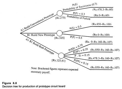
It is because the total cost is Rs. 160,000 which is much less than the budgetary limit of Rs. 400,000. However, if both the prototypes are developed, an additional labour cost of Rs.107,000 has to be incurred. Fig. 8.8 presents the decision tree associated both the problem faced by Mr. Ram.
If the maximization of EMV criterion is followed, the decision would be to build both prototypes because the expected profits of Rs. 325,410 would far exceed the profit of any one of the two.
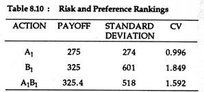
However, in order to measure the riskiness of the three alternatives, Mr. Ram computes the standard deviation of each of the alternatives. Moreover, he computes coefficient of variation to make a comparison of the degree of riskiness of the three actions.
The results of such computations are presented in Table 8.10 below:
It is clear that construction of the prototype using conventional materials (A1) is the least risky alternative. But its payoff is also the lowest of the three. Hence Mr. Ram is faced with a perplexing dilemma — a trade-off between risk and profitability. Larger return implies higher risk.
vi. Adjusting the Valuation Model for Risk:
Diminishing marginal utility of money leads directly to risk aversion. Such risk aversion is reflected in the valuation model used by investors to determine the worth of a firm. Thus, if a firm succeeds in taking an action that increases its risk level, this action affects its value.
The model was introduced as a way of discounting future income stream to the present:
Where Rt = sales revenue from Qt units;
Ct = cost of producing Qt units;
Πt = profit;
r = interest rate; and
t = time period under consideration; t equal to zero in base (current) year and n at the end of n time periods.
The model, it may be recalled, states that the value of a firm to its investors is the discounted present worth of future profits or income. Under uncertain conditions the profits in the numerator, Rt – Ct = Pt, are really the expected value of the profits each year.
If the firm has to choose between alternative methods of operation, one with high expected profits and high risk and another with smaller expected profits and lower risk, will the higher expected profits be sufficient to neutralize the high degree of risk involved in it? If so, the riskier alternative will surely be preferred; otherwise the low-risk project or method of operation should be accepted.
We devoted ourselves to developing a broad understanding of the economic aspects of the NPV equation. We noted that an economic organization seeks to maximize its prospects for economic survival by maximizing NPV.
Now we shall interpret our valuation model of the firm in terms of the expected utility approach. The switch-over from utility theory to the NPV model is a simple exercise. Because of the diminishing marginal utility of money most decision-makers (e.g., investors) are risk averters.
Now, in the context of our NPV model we may assert that risk aversion is reflected in the fact that any decision that a firm makes will surely change its risk level — the degree of risk to which it is exposed. The change in the risk level because of the decision taken by the firm will have a direct bearing on its NPV level. Now an important question is: how to adjust our basic valuation model for risk?
There are two ways of adjusting the model in the light of reality, i.e.,:
(1) Using the concept of certainty equivalent and
(2) Using risk- adjusted discount rate.
Decision-Making Environment under Certainty Equivalents:
The first method of dealing with risk it to replace the expected net income figures (Rt — Ct) in the NPV equation with their certainty equivalents.
We may now illustrate the concept. Suppose Mr. Hari has purchased a lottery ticket that has a 50-50 chance of paying Rs. 1,000 or Re. 0. Thus the lottery is equivalent to tossing an unbiased coin. If head appears, Mr. Hari will get Rs. 1,000 and if tail appears he gets nothing. If we adopt the classical definition of probability as the limit of relative frequency, we know one thing at least.
If Mr. Hari tosses the coin again and again, on an average, he would win (get a head) half the time and lose (get a tail) half the time. Thus Mr. Hari’s average or expected payoff in this game is Rs. 500 per ticket. This much is known to us.
But what we do not know as yet is; how much would Mr. Hari be willing to sell his ticket for? To put the question in a different language, what is the lowest offer that Mr. Hari is willing to accept — Rs. 300, Rs. 500 or Rs. 600? The cash offer he would accept in order to be induced to part with his ticket is the certainty equivalent (CE) of the lottery.
If, for instance, he would accept Rs. 300 (CE = Rs. 300), then his risk premium (RP) can be defined as:
RP = EMV- CE
Rs. 200 = Rs. 500 – Rs. 300 (8.18)
In such a situation Mr. Hari is willing to pay Rs. 200 risk premium to quit (sell the lottery ticket). Since his CE is less than his EMV, the risk premium is positive and he would be classified as a risk-averter. Had his CE exactly equalled the EMV of Rs. 500, he would be described as risk- neutral (indifferent).
Alternatively, he may be a risk-lover, in which case he would not exit the game (part with the lottery ticket) unless he received more than Rs. 500. On the basis of this simple example, we may define CE of a decision as “the sum of money, available with certainty, that would cause the decision-maker to be indifferent between accepting the certain sum of money and making a decision (or taking the gamble)”.
It is obvious that CE sum equal to the EMV implies risk indifference. Likewise, a CE sum greater than the EMV indicates risk. Therefore, an individual’s attitude toward risk is directly reflected in the CE adjustment factor.
It is calculated as the ratio of the equivalent certain rupees sum (i.e., the certain sum whose utility is equal to the expected utility of the risky alternative) divided by the expected rupee outcome from the risky alternative as equation (8.18) shows.
α = Equivalent Certain Sum/Expected Risky Sum
Let us suppose that Zt represents the CE for net income (Rt – Ct) in period t.
Now the NPV equation may be rewritten as:
The calculation of the certainty equivalent (Zt) could be done on a purely subjective basis by the individual carrying out the financial analysis, or the analyst could make use of a formal estimate (based on actual information and an appropriate model). If we substitute the value of Zt in equation (8.19), the NPV calculation would reflect a crude adjustment for risk.
It may be emphasized at this stage that the process of adjusting for time and risk in the NP V model is a complex and controversial task. In fact, even the order (risk first or time first) in which one adjusts the cash flow (numerator in the NPV model) can have a major impact on the final results.
The most obvious defect of the CE approach, outlined above, is that it requires the specification of a utility function so that risk premium can be numerically measured or quantified. However, one way possible of overcoming this problem is to go through an alternative and better known risk adjustment process — the risk adjusted discount rate method.
The Risk Adjusted Discounted Rate (RADR):
The RADR approach is very easy to use and therefore very popular. In order to understand the concept let us go back to equation (8.16). Recall that the CE approach to adjusting our basic valuation model to risk operated on the numerator (Rt — Ct). By contrast, the RADR method focuses on the denominator.
To be more specific, the RADR procedure replaces the discount rate with a new term p, which is the sum of the initial discount rate and risk factor k. That is p = r + k. If, for instance, r equals 10% and k equals 3%, the new risk-adjusted discount rate becomes 13%.
Increasing the discount rate implies deflating NPV. Since NPV analysis uses a compounding factor in the denominator (1+r)t the incorporation of a risk adjustment factor in the denominator to deflate future values, heightens this compounding.
To illustrate, a discount rate of 10% becomes a discount factor of 1.46 [= (1.10)4] by the end of four years, and the 13% rate becomes 1.63 [=(1.13)4].
However, there is hardly any justification for the assumption of a compounding risk factor, rather than a risk difference of just three percentage points (1.13 – 1.10) or a ratio of (1.63 – 1.46=) 1.116 by the end of four years. Thus, the risk differential increases with the number of years in the project.
This particular observation has important implications for project planning and long-term investment decision. If, for example, there are two investment projects with the same degree of risk but differing time horizons, then the use of a common discount rate (such as 13%, in our example) is sure to have a distorting influence for the longer project.
The reason is simple enough: the risk factor will continue to compound in later years. However, the RADR is not without its defects. Its major defect is that, as one number, the discount rate is used to combine the effects of both risk and the time value of money.
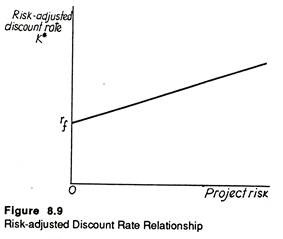
The RADR is often made us of in capital budgeting (i.e., long-term investment) decisions. If this factor is brought into consideration, future cash flows for each project are discounted at a rate, K*, which is based on the risk associated with the project. Fig. 8.9 illustrates the relationship between K* and project risk.
Here the rƒ value denotes the risk-free rate, i.e., the minimum acceptable rate of return from an investment project having certain cash flow streams. Fig. 8.9 makes one point clear at least: the greater the project risk the higher the rate used in discounting the project’s cash flows.
Decision under Conflict and Game Theory:
So far we have considered only a single decision maker. The states of nature occur passively and independently of the strategies chosen. When opponents are involved, the opponents’ strategies can be represented by the columns.
These will replace the states of nature and there will be as many columns as strategies. The two decision-makers will not choose their strategies independently. There will be interaction, the basis of which is conflict of interest.
Decision theory involving 2 or more decision makers is known as game theory. Games are classified according to number of players and degree of conflict of interest.
With complete conflict of interest the game is a zero-sum game. Most parlour games are of this type. A duopoly battle to capture a higher share of the market is another. If the conflict of interest is not complete, the game is called a non-zero sum game. With external economies, such games could arise.
Let us consider a decision problem facing two players. Both players wish to maximise their payoffs. Player A has 3 and player B has 4 strategies. For example, 3 multinationals want contracts in a Banana Republic. The first company could either bribe the present government, arranging a coup invasion. The second company has an extra option of getting a neighbouring country to attack. The payoffs are measured in terms of profit.
With a zero sum game, player A’s gain is B’s loss. Therefore a single matrix can represent both players payoffs. Payoff to B = – (Payoff to A).
If A chooses strategy A1, B will try to maximise his own payoff (that is, minimise A’s payoff). So B will choose B2 . Similarly if A chooses A2, B will choose B3. If A chooses A3, B will chose B1. So the relevant payoffs for each strategy is the minimum for each now. A will maximise this and choose A2. This is nothing but the maximin criterion.
Whatever strategy B chooses, A will try to maximise his own pay-offs. So if B chooses B1, A chooses A1 and so on.
B will choose strategy B3. This minimises A’s payoff and therefore maximises his own. So B chooses the minimax criterion. In this case the payoffs under minimax and maximin principles are the same and equal to 1.5. If this happens, such a value is called a saddle point. It is the solution to the game.
But even if no saddle point exists, a solution to any zero-sum-two person game will exist. The solution will be in terms of mixed strategies (where the specific strategy to be used is selected randomly with a pre-determined probability). The proof of this is known as the fundamental theorem of game theory.
It is sometimes difficult to get the exact utilities required to construct a payoff matrix. Ranked data are then often used. The two competitors may not have the same approximate utilities (with a negative sign). The two payoff matrices will be required. It will also be necessary to assume that each competitor can estimate the other’s utility. It is the existence of such dissimilar utilities that cause non-zero-sum type of games.
It may also be that the opponent’s utilities are not known at all: The decision problem would then have to be treated under uncertainty. Not knowing the opponent’s utilities implies that the player has no idea at all about the possible choice of strategies that is equivalent to decision-making under uncertainty for a single decision-maker.
In terms of actual conditions a large number of problems is involved with states of nature. Even with situations involving antagonistic decision makers, this analysis is often not applicable under perfect competition.
The activities of a single entrepreneur will not then affect market conditions. But whenever a single firm controls a large share of the market, either with duopoly or oligopoly, game theory becomes important. Even monopoly can be represented as a game between a producer and seller.
