Role of Government in Externalities Production

In this article we will discuss about the Role of Government in Externalities Production.

External­ities exist, costs and benefits are not truly reflected in market prices. In such circumstances, produc­tion according to marginal cost pricing (i.e.. to set output at a level where marginal costs, MC, equals marginal revenue, MR) leads to misallocation (or inefficient allocation) of resources, and hence Pareto Optimality is violated.

Suppose, a producer is selling in a perfectly competitive market and he is following the profit- maximization motive. Let his cost function be rep­resented by C_i = C_i (q₁, q₂); where is the output of the i-th producer (assume that there are only two producers so that i = 1, 2); that q₂ is an argument of C_i implying that the first producer is facing ex­ternal effects (as output level of the second producer influences the first’s costs).

However, suppose that the first producer is either totally ignorant of this ef­fect or he simply does not care about it.

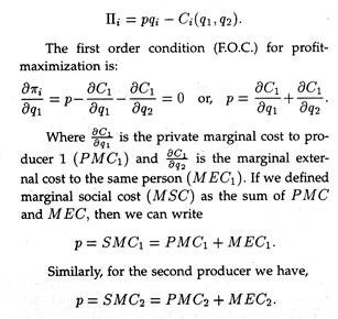
If π_i, is the profit of the i-th producer and p be the given market price, then we obtain:

 

 

 

 

 

 

 

 

 

 

 

And there exist external economies or disecono­mies to producer i according as MEC_i < 0. Sup­pose, the first individual experiences external dis­economies. Then MEC₁ > 0. Here SMC₁ > PMC₁.

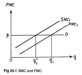
In Fig 25.1 we have represented SMC₁ and PMC₁ curves (note, under perfect competition the rising portions of the MC curves above the average variable cost curves give the firms supply curves). Here pD is the demand (which in perfect competi­tion is also the marginal revenue, MR) curve.

Producer 1 ignores MEC₁. Therefore, he sets output at q’₁ where PMC₁ = p. However, had he taken care of external effects, he would have set out­put at a level where p = SMC and this occurs at an output level of q”₁. At q’₁ level of output, Pareto Optimality is violated; therefore, producer 1 is over­producing (which is more than the socially desirable level q”₁) and so there is a misallocation of resources.

The production of liquor is a nice example of this phenomenon. The liquor producer only considers PMC₁; but-ignores MEC arising out of pollution, accidents caused by drunk (consumers) drivers, etc. Had he taken these external costs into consideration, he would produce less liquor and society would be better off.

Still p = SMC does not necessarily guaran­tee the production of socially desirable output level; it may well be the case that social marginal ben­efit (SMB) is not fully reflected in price so that p ≠ SMB. Social optimality requires that SMB = P = SMC. If p < SMB, then output remains at less than socially optimal level.

In this case, con­sumers receive an external benefit, but do not pay for it; if the price of the external benefits is appro­priated from them, output will increase and it will be supplied at a level where SMB = SMC.

In an n-good economy, the overall optimality condition can be written as:

 

 

 

The situation reverses when for producer 1,

MEC₁ < 0 so that SMC₁ < PMC₁. Here SMC₁ lies uniformly below PMC₁; hence, if the external effects (external economies) are considered, greater output will be generated if price is set equal to SMC. On other hand, if p = SMC, but p = SMC > SMB, then a negative external effect exists and consideration of this effect will lead to a lower out­put level, which is socially desirable.

We thus see that production externalities (when they are ignored) lead to over or under production and this results in a sub-optimal social gain (or ben­efits). Let us illustrate this with a formal example.

Let the cost functions of the two producers be:

where q_i and C_i are output and cost of the i-th pro­ducer (or firm). Let the price be p = Rs. 80 per unit of output (note, the market is perfectly com­petitive).

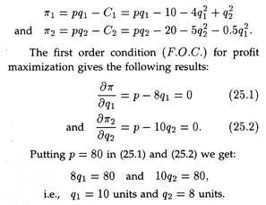
It is evident from the cost functions that there are external economies. Firm 1 creates exter­nal diseconomies for Firm 2, and receives external economies generated by Firm 2, i.e., ∂c₁/∂q₂ < 0 and ∂c₂/∂q₂ > 0. Suppose, both firms are ignorant about ex­ternalities and hence equates respective PMC and MR(= p) to maximize profit (π). Then

Hence, π₁ = Rs. 454 and π₂ = Rs. 250. So the combined profits is π = (π₁ + π₂) = Rs. 704. We now proceed to show that in this case, so­ciety’s gain (if we take profit as the indicator) will be maximized (and hence social optimality will be attained) if the two firms decide to maximize joint profit.

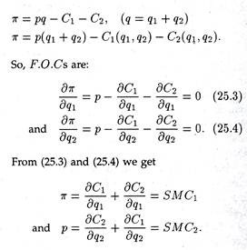
Now

 

 

 

 

 

 

 

 

 

 

 

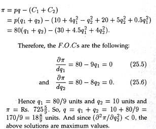
Since SMC₁ = p = SMC₂ joint profit maxi­mization leads to optimal resource allocation. Now, let us carry out the same exercise for our hypothet­ical firms.

 

 

 

 

 

 

 

 

 

 

It is now evident that combined profit Rs. 725 5/9 is greater than previous total profits Rs. 704, com­bined output of 18 8/9 units is also greater than the earlier total 18(= 10 + 8).

It is also confirmed that reduce its output from 10 units to 80/9 units, (note that the first firm is the cause of external diseconomies) and has encouraged the second firm (the creator of external economies) to raise its output level from 8 units to 10 units.

We see then that in the presence of externali­ties the production of the firm causing diseconomies should be discouraged and that of the firm creat­ing economies should be encouraged.

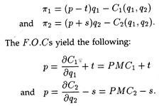
If the two firms fail to reach a mutual settlement, the government has to intervene to secure socially optimal re­source allocation. To discourage production of Firm 1 and encourage production of Firm 2, the govern­ment should tax the former and subsidize the latter. Let t be unit tax and s be the unit subsidy.

Now we have:

 

 

 

 

 

 

Therefore, to make p = SMC, optimal ‘t’ should be equal to ∂c₂/∂q₁ and ‘s’ should be equal to ∂c₁/∂q₂ . In our example, after government intervention, we get

(i.e., each producer sets PMC equal to p; note here that unit tax can be treated as a portion of total vari­able cost, and subsidy as negative cost).

Putting q₁ = 80/9 and q₂ = 10 in (25.7) and (25.8) respectively, we estimate optimal tax and sub­sidy rates as follows:

If q*_i is the post-tax subsidy level of production for the i-th producer, the net government expendi­ture is

E = sq*₂ –  tq*₁

Where sq*₂ is total expenditure on account of subsidy and tq*₁ is total revenue from tax. If E > 0, i.e., payments exceed receipts, problem arises.

The government can avoid this problem by charging a lump-sum profit tax on Firm 1, because a lump-sum profit tax leaves optimal price-quantity combination unaltered. In our case, E = [20.10 – (80/9) (80/9)] = (200 – 6400/81) = Rs. 120 80/81. So, our hypothetical case entails an imposition of lump-sum profit tax on Firm 1 to bridge the gap between payments and receipts.

Increasing Returns and Government Inter­vention:

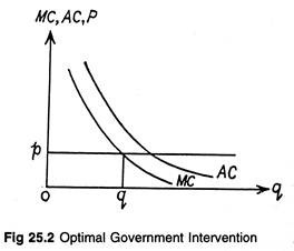
Suppose, due to some external effects, firm fac­ing perfect competition is subject to increasing re­turns to scale (i.e., decreasing cost). In this case MC will be uniformly below the AC (average cost) curve at all output levels (see figure 25.2). If our pro­ducer is guided by marginal-cost pricing (MCP), then P = MC < AC.

Hence, he incurs losses at all levels of production. Under such circumstances if production is to be maintained, either the govern­ment will have to subsidize the producer, or it will have to take over the production process itself.