Shifts of IS & LM Curves (With Diagram)

In this article we will discuss about the shifts of IS & LM curves, explained with the help of suitable diagrams. Also learn about the cause and effect of such shifts.

Any fiscal policy change (a change in government expenditure or taxes) will shift the IS curve. Similarly, any monetary policy change will shift the LM curve.

Shifts of the IS Curve:

As a result of changes in government spending, both income and interest fate respond positively, increase in taxes or reduction in government expenditure or both reduce the level of income and thus shifts the aggregate expenditure curve downwards.

Thus, an increase in taxes shifts toe IS curve to the left. National income falls in the commodity market. The demand for money is reduced in the money market and as a consequence toe rate of interest falls. So, at the end the rate of interest and the level of income both fall.

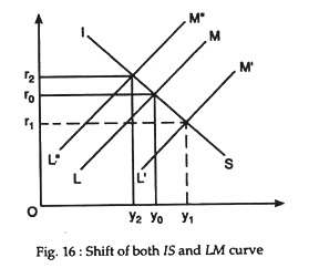
Conversely, a reduction in taxes or an increase in government expen­diture or both fall. Conversely, a reduction in taxes or an increase in government expenditure or both shift the IS curve to the right (Fig. 16) and raise both Y and r.

Shifts of the LM Curve:

An increase in money supply shifts the LM curve to toe right and reduces toe rate of interest. This raises investment in the commodity market. Income consequently rises. Similarly an increase in the demand for money, for instance, raises the rate of in­terest by shifting the LM curve leftward (Fig.16); in­vestment falls and so income.

All these shifts make it clear that the two markets — the commercial market and money market of the econo­my are inter-related. And the IS-LM model seeks to study the nature of this interdependence.

Shifts of Both the Curves:

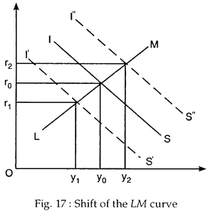
If both curves shift at the same time, the consequence is unpredictable Consider Fig. 17. If IS curve shifts to the right and LM curve to the left the rate of interest increases (from r₀ to r₁), but income remains unchanged (at Y_e). Al­ternatively, if both shift to the right, the rate of interest re­mains unchanged (at r₀), but the level of income rises (from Y₀ to Y₁).

Suppose, due to a cut in taxes the IS curve shifts to the right. The new equilibrium point is E’ which shows a higher rate of interest and a higher level of income. Now, if the government increases money supply the LM curve shifts to the right (L” M”) The new equilibrium point is E”. So, the level of income is higher now at an unchanged rate of interest.

Monetary policy can neutralise the ad­verse effects of fiscal policy and bring about the desired change in the economy. We can also think of other possibilities. Thus, by making appro­priate use of monetary and fiscal measures it is possible to achieve the desired goals of the economy such as full employment and price level stability. See table below.