How does a Monopolist Determine Price and Output?

Equilibrium of a Monopolist:

The goal of a monopolist is also profit maximization.

In order to attain maximum profit or, in order to be in equilibrium, the following two conditions are to be fulfilled:

Firstly, MC must be equal to MR. This condition is known as necessary condition or first-order condition (FOC) for equilibrium.

Secondly, the slope of MC curve must be greater than the slope of MR curve. This condition is called sufficient condition or the second-order condition (SOC) for equilibrium. Only when these two conditions are satisfied simultaneously does a monopoly firm reach equilibrium—irrespective of time period.

(a) Short Run Equilibrium:

A monopolist faces a negative sloping demand curve or AR curve. If he wants to sell more he must lower the price of his product. The corresponding MR curve is also downward sloping and lies below the AR curve i.e., AR > MR.

As a firm behaves as a price-taker under perfect competition, its only concern is output determination. Price is given to a firm. But since a monopolist is a price-setter he must take both price and output decisions. However, given the downward sloping demand curve, these two decisions are interdependent; fulfilment of one decision leads to the fulfilment of the other.

That is why the monopolist will either set the price or sell the amount that the market will absorb or determine output which will be sold at the corresponding price. What is essential for profit-maximization is the fulfilment of both FOC and SOC. Under monopoly, like perfect competition, the ‘golden rule of output’ determination is MC – MR equality.

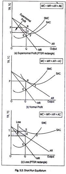
A monopolist, in the short run, can earn pure profit or economic profit as well as normal profit. A monopolist may also incur a loss in the short run. All these possibilities have been shown in Fig. 5.2. The equilibrium point is E. Corresponding to this equilibrium point, the monopolist produces OQ output and sells it at a price OP.

Fig. 5.2(a) demonstrates that a monopolist earns pure profit since TR from the sale of OQ output (i.e., OPRQ) exceeds total cost (i.e., OTSQ). Thus, the area TSRP is the area of supernormal profit. A monopolist earns supernormal profit when

MC = MR < AR > AC

That is to say, if AC curve lies below the demand curve the monopolist will enjoy supernormal profit.

Fig. 5.2(b) shows normal profit since TR (i.e., OPRQ) equals TC (i.e., OPRQ).

The condition for normal profit is, thus,

MC = MR < AR = AC

That is to say, normal profit is enjoyed by the monopolist when AC curve at a particular point coincides with the AR curve.

There is a misconception that a monopolist always earns supernormal profit and does not suffer from loss. A monopolist may also incur a loss, of course in the short run. Fig. 5.2(c) shows that the monopolist suffers a loss of PRST amount since TC (i.e., OTSQ) exceeds TR (i.e., OPRQ). A situation of loss will arise when

MC = MR < AR < AC

In other words, if AC curve lies above the AR curve at the corresponding level of output, the firm will suffer a loss. However, a monopolist will continue production in the short run (i.e., minimizes losses) if he covers up only AVC. In other words, if the loss of the monopolist is equivalent to fixed cost he will stay in business.

Loss then amounts to only fixed cost. But, if the monopolist fails to cover up variable cost, i.e., if P < AVC, only then will he suspend production. He will ‘drop out’. Of course, there cannot be loss in the long run.

(b) Long Run Equilibrium:

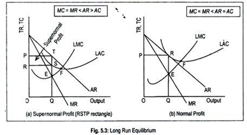
In the long run, the monopolist can change his scale of production so that profit becomes the highest. Since entry is blocked, excess profit will be enjoyed by the monopolist. A monopolist also earns normal profit in the long run but does not incur a loss. Fig. 5.3 demonstrates these two possibilities.

In Fig. 5.3, LAC and LMC are the long run average cost and long run marginal cost curves. Corresponding to the equilibrium point E, the monopolist produces and sells OQ output at the price OP. Fig. 5.3(a) shows a situation of supernormal profit to the extent of RSTP since costs are lower then revenue, i.e.,

MC = MR < AR > AC

On the other hand, Fig. 5.3(b) demons­trates normal profit situation since

MC = MR < AR = AC

Important Points about Monopoly Equilibrium:

In the first place, a monopolist always produces at the elastic range of his demand curve. Or a monopolist never operates at the inelastic range of his demand curve. The basic goal of the monopolist is the maximization of profit. Profit becomes maximum when the FOC and SOC for equilibrium are satisfied.

FOC states that a monopolist attains equilibrium when MC equals MR. We know that MR = AR (1 – 1/e). If the coefficient of elasticity of demand becomes greater than one (i.e., e > 1) at a particular point of a straight line demand curve, MR becomes positive. Costs are always positive.

Equili­brium must occur when positive MC equals positive MR. But, if the coefficient of elasticity of demand is less than one (i.e., e < 1), MR will be negative. Negative MR can never be equated with positive MC. Thus, in this range of demand curve, a monopolist cannot reach equilibrium. Finally, when the coefficient of elasticity of demand is unity (i.e., e = 1), MR will be zero.

Equilibrium cannot be attained even in this case since positive MC cannot be matched with the zero MR. So, a monopolist will not also produce in this range of demand curve. In other words, a monopolist always operates at the elastic range (i.e., e > 1) of his demand curve to obtain maximum profit.

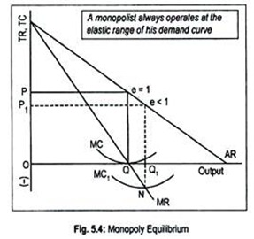
Let us explain these two situations in terms of Fig. 5.4. If coefficient of elasticity of demand is one, MR becomes zero. Therefore, to reach equilibrium, MC must be zero. This happens at OQ output where MC equals MR. The monopolist sells OQ output at price OP.

But zero marginal cost is hardly conceivable. Again, if e < 1, MR will be negative. Equilibrium requires MR-MC equality. Since MR is negative, MC must be negative.

It is clear from the figure that the monopoly firm reaches equilibrium at point N (i.e., the negative quadrant) and it produces OQ₁ output and sells it at a price OP₁. But negative MC is hard to imagine. Therefore, the monopolist will always operate at the elastic range of his demand curve where both MC and MR become positive.

Secondly, a monopolist never operates at the lowest point of his AC curve where cost becomes the least. Actually, he operates somewhere to the left of the minimum point of his AC curve, be it in the short run or in the long run. In Figs. 5.2 and 5.3, the lowest point of AC curve has been represented by the point F.

Consider Fig. 5.3(b) where the monopoly firm operates at point R—a point to the left of point F—the lowest point of the LAC curve.

This happens due to the nature of the demand curve. As the demand curve is downward sloping it must be tangential to the falling portion of AC curve. Operation at this point implies that the monopoly firm cannot utilize its plant optimally. Or it implies under-utilization of resource.

As entry is closed, there is no urgency of a monopoly firm to operate at the lowest point of AC curve. However, a competitive firm always operates at the lowest point of its AC curve since demand curve is perfectly elastic.

However, some economists have suggested that, in the long run, a monopoly firm may not only operate to the left of the minimum point of AC curve (i.e., sub- optimal scale), but may also operate at the lowest point of AC curve (i.e., optimal scale) and may also operate to the right of the minimum point of AC curve (i.e., over- optimal scale) depending on the extent of market or demand for the monopoly product.

This means that demand for the monopoly product is such that it is profitable on the part of the monopolist in the long run to operate at the minimum point of AC curve or to the right of the minimum point of the AC curve.