Equilibrium of a Firm under Monopolistic Competition | Markets

In this article we will discuss about the equilibrium of a firm under monopolistic competition.

Assumptions of Equilibrium Analysis of a Firm:

The equilibrium analysis of a firm under monopolistic competition is based on the following assumptions that are peculiar to monopolistic competition.

(i) The firms here produce products of the product-group, each producing one particular product.

(ii) They share the total market for the product-group equally.

(iii) They are equal in respect of cost of production and also in respect of their reactions to changes in different parameters.

Apart from the above assumptions, there would also be present in our analysis the usual assumptions such as those of the profit-maximising goal of the firms and of the third degree and second degree shapes of the total, average and marginal cost curves.

Equilibrium of the Firm in the Short Run:

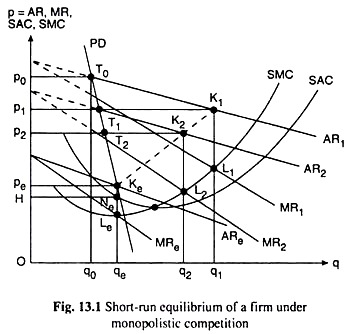
We shall explain the short-run equilibrium of an individual firm under monopolistic competi­tion with the help of Fig. 13.1, where SAC and SMC are the short-run average and marginal cost curves of the firm. On the demand side, if there are n firms, each firm would be able to sell, by assumption, 1/nth part of the market demand for the product-group at any particular price.

This is shown by what is known as the proportional demand (PD) curve. This curve is given by the curve PD in Fig. 13.1.

Now, given the PD curve, let us start from a short-run disequilibrium position where the price is p₀. At p = p₀, the firm would be able to sell the output q = q₀, which is the amount of proportional demand, i.e., which is equal to 1/nth part of the total demand for the product-group at the said price.

However, according to the perception of the firm, if the price of its product decreases from p = p₀, the prices of all other products of the group remaining unchanged, then the quantity demanded of its product (q) would increase more than that along the PD curve—it would increase along a flatter demand curve like AR.

This curve is known as the firm’s ‘perceived’ demand or AR curve. All the ‘perceived’ AR and MR curves have been drawn as straight lines in Fig. 13.1, for the sake of simplicity. The marginal curve of AR₁ is MR₁.

The firm thinks that it would be able to maxim­ise profit at the MR = MC point which is the point L₁ in this case. At L₁, the profit-maximising price-output combi­nation is (p₁, q₁) which is obtained at the point K₁ on the AR₁ line.

Now, as the firm sets p = p₁, it would be able to sell not q = q₁ > PD, but q = p₁T₁ = PD, T₁ being a point on its PD curve. This would be so, because, as the firm decreases the price from p₀ to p₁, all other firms react in the same way, by assumption, i.e., all other firms also would reduce the prices of their products to p = p₁.

It follows then that, at p = p₁, when the firm sells q = p₁T₁ and not q = q₁, it would not be able to maximise profit. Therefore, the firm would again want to move along its ‘perceived’ demand curve, which is now obtained to be the line AR₂. The marginal curve for AR₂ is the line MR₂. The MR = MC point, now, is L₂ and the corresponding profit-maximising price-output combination is K₂(p₂, q₂) on the AR₂ line.

However, as before, the firm’s goal of profit-maximisation would not be achieved at p = p₂, because, all other firms would charge now the same price and each firm (and our firm also) would now be able to sell not q = q₂ > PD, but q = p₂T₂ = PD, where T₂ is a point on the PD curve.

Since, at the point T₂, the firm is still in a disequilibrium position, it would now try again to achieve its profit-maximising goal, and the process would go on.

It is now clear, from the above analysis that the firm would be moving from one ‘perceived’ equilibrium to another along a path shown by the dotted line passing through K₁, K₂, etc. in Fig, 13.1 till its ‘perceived’ equilibrium combination, while moving along the said dotted line, reaches the PD curve at a point like K_e(p_e, q_e).

Now, every point on the dotted line lies on some ‘perceived’ AR curve and, for this point, we also have MR = MC.

Therefore, K_e must be a point on some AR line which is, let us suppose AR_e, and for the point K_e or at q = q_e, we have MR = MC at the point L_e. K_e(p_e, q_e), therefore, is a ‘perceived’ profit-maxim­ising (p, q) combination at which the firm would be willing to sell q = q_e at p = p_e.

However, since the point K_e lies on the PD curve, the firm would be able to sell actually q = q_e at p = p_e. That is, K_e (p_e, q_e) would be the ‘perceived’ profit-maximising price-output combination where the goal would be realised also. In other words, the firm is in short-run equilibrium at the MR = MC point L_e and its equilibrium (p, q) combination is K_e(p_e, q_e).

It is seen in Fig. 13.1 that at this equilibrium point the firm’s AR = K_eq_e is greater than its AC = N_eq_e which gives us that in this short-run equilibrium, the firm would be able to earn more than normal profit. The amount of excess profit here is equal to □p_eK_eN_eH.

Long-Run Equilibrium of the Firm and the Group under Monopolistic Competition:

We have to explain how the firm and the group under monopolistic competition reach the position of long-run equilibrium and what are the characteristic features of this equilibrium.

But before doing this, let us remember that the short run equilibrium of a firm under monopo­listic competition occurs when the price-output combination corresponding to the perceived MR = MC point is a point on its perceived demand (AR) curve where this curve intersects the proportional demand (PD) curve. This point is the point K_e in Fig. 13.1.

Now if the firm happens to earn excess profit at this point of short-run equilibrium as it does in Fig. 13.1 (since P = AR > AC), then in the long run, by assumption, the number of firms in the group under monopolistic competition rises.

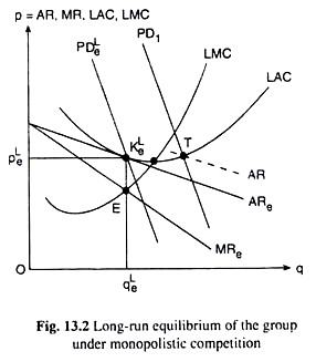
As the number of firms starts rising in the long run, the PD curve of each firm begins to shift to the left. Because the market for the product-group now gets divided among larger and larger number of firms. For example, in Fig. 13.2, a particular long run disequilibrium position of the PD curve is given by PD₁. At every point of the PD curve (like PD₁) the firm may have a per­ceived demand (AR) curve.

Now, as the number of firms increases in the long run, the PD curve along with the perceived demand curves shifts to the left. The process goes on till the number of firms happens to be so large that the PD curve, while shifting to left, comes to a position like PD^L_e and intersects the LAC curve of the firm at a point like K^L_e in Fig. 13.2 and, at this point, the perceived demand curve, AR_e, touches the LAC curve.

At the point K^L_e, the number of firms is so large that each firm reaches the position of normal-profit-earning long run equilib­rium.

For at this point we obtain:

(i) AR = LAC and so, this firm earns just the normal profit;

(ii) The firm wants to sell q = q^L_e at p = p^L_e, and the firm is actually able to sell this quantity, because the (p^L_e, q^L_e) combination lies on its PD curve, viz., PD^L_e; and

(iii) Since TR and LTC curves (not shown in Fig. 13.2) would also touch each other at this output, we have MR = LMC at q= q^L_e. That is why the profit-maximising firm wants to sell q= q^L_e at the AR = LAC point, K^L_e.

It may be noted here that if the perceived demand curve, like the dotted AR curve in Fig. 13.2, does not touch the LAC curve at the point of intersection, T, between the PD curve and the LAC curve, the firm would not come to an MR = LMC position although it is at an AR = LAC position; and so the process continues till a point like K^L_e is obtained.

When all the firms are in long-run equilibrium at the point like K^L_e in Fig. 13.2. the group under monopolistic competition will also be in long-run equilibrium—since all the firms are earning just the normal profit, there would be no tendency for the new firms to join the group.

It may be noted here that if the firms under monopolistic competition happen to earn less than normal profit in the short run, then in the long run some of the existing firms would be leaving the group, and the PD curve would be shifting to the right, till the existing firms are in a position to earn the normal profit. At this point the firms and the group will be in long-run equilibrium.