Determining the Price and Equilibrium of a Firm under Monopoly

Under monopoly, for the equilibrium and price determination there are two different conditions which are:

1. Marginal revenue must be equal to marginal cost.

2. MC must cut MR from below.

However, there are two approaches to determine equilibrium price under monopoly viz.;

1. Total Revenue and Total Cost Approach.

2. Marginal Revenue and Marginal Cost Approach.

Total Revenue and Total Cost Approach:

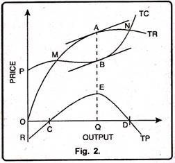
Monopolist can earn maximum profits when difference between TR and TC is maximum. By fixing different prices, a monopolist tries to find out the level of output where the difference between TR and TC is maximum. The level of output where monopolist earns maximum profits is called the equilibrium situation. This can be explained with the help of fig. 2.

In Fig. 2, TC is the total cost curve. TR is the total revenue curve. TR curve starts from the origin. It indicates that at zero level of output, TR will also be zero. TC curve starts from P. It reflects that even if the firm discontinues its production, it will have to suffer the loss of fixed costs.

Total profits of the firm are represented by TP curve. It starts from point R showing that initially firm is faced with negative profits. Now as the firm increases its production, TR also increases. But in the initial stage, the rate of increase in TR is less than TC.

Therefore, RC part of TP curve reflects that firm is incurring losses. At point M, total revenue is equal to total cost. It shows that firm is working under no profit, no loss basis. Point M is called the breakeven point. When firm produces more than point M, TR will be more than TC. TP curve also slopes upward. It shows that firm is earning profit. Now as the TP curve reaches point E then the firm will be earning maximum profits. This amount of output will be termed as equilibrium output.

Marginal Revenue and Marginal Cost Approach:

According to marginal revenue and marginal cost approach, a monopolist will be in equilibrium when two conditions are fulfilled i.e., (i) MC=MR and (ii) MC must cut MR from
below. The study of equilibrium price according to this analysis can be conducted in two time periods.

1. The Short Run

2. The Long Run

1. Short Run Equilibrium under Monopoly:

Short period refers to that period in which the monopolist has to work with a given existing plant. In other words, the monopolist cannot change the fixed factors like, plant, machinery etc. in the short period. Monopolist can increase his output by changing the variable factors. In this period, the monopolist can enjoy super-normal profits, normal profits and sustain losses.

These three possibilities are described as follows:

Super Normal Profits:

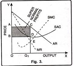
If the price determined by the monopolist in more than AC, he will get super normal profits. The monopolist will produce up to the level where MC=MR. This limit will indicate equilibrium output. In Figure 3 output is measured on X-axis and price on Y-axis. SAC and SMC are the short run average cost and marginal cost curves while AR or MR are the average revenue or marginal revenue curves respectively.

The monopolist is in equilibrium at point E because at point E both the conditions of equilibrium are fulfilled i.e., MR = MC and MC intersects the MR curve from below. At this level of equilibrium the monopolist will produce OQ₁ level of output and sells it at CQ₁ price which is more than average cost DQ₁ by CD per unit. Therefore, in this case total profits of the monopolist will be equal to shaded area ABDC.

Normal Profits:

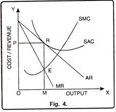
A monopolist in the short run would enjoy normal profits when average revenue is just equal to average cost. We know that average cost of production is inclusive of normal profits. This situation can be illustrated with the help of fig 4.

In Fig. 4 the firm is in equilibrium at point E. Here marginal cost is equal to marginal revenue. The firm is producing OM level of output. At OM level of output average cost curve touches the average revenue curve at point P. Therefore, at point ‘P’ price OR is equal to average cost of the total product. In this way, monopoly firm enjoys the normal profits.

Minimum Losses:

In the short run, the monopolist may have to incur losses. This situation occurs if in the short run price falls below the variable cost. In other words, if price falls due to depression and fall in demand, the monopolist will continue to produce as long as price covers the average variable cost. Once the price falls

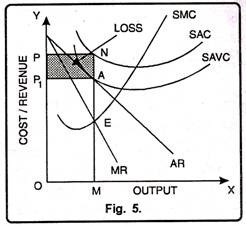
Below the average variable cost, monopolist will stop production. Thus, a monopolist in the short run equilibrium has to bear the minimum loss equal to fixed costs. Therefore, equilibrium price will be equal to average variable cost. This situation can also be explained with the help of Fig. 5.

In Fig. 5 monopolist is in equilibrium at point E. At point E marginal cost is equal to marginal revenue and he produces OM level of output. At OM level of output, equilibrium price fixed by the monopolist is OP₁. At OP1 price, AVC touches the AR curve at point A.

It signifies that the firm will cover only average variable cost from the prevailing price. At OP₁ price, firm will bear loss of fixed cost i.e., A per unit. The firm will bear the total loss equal to the shaded area PP₁ AN. Now if the price falls below OP₁, the monopolist will stop production. It is so because if he continues production, he will have to bear the loss of variable costs along with fixed costs.

2. Long Run Equilibrium under Monopoly:

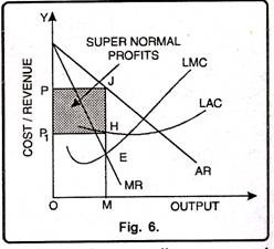
Long-run is the period in which output can be changed by changing the factors of production. In other words, all variable factors can be changed and monopolist would choose that plant size which is most appropriate for specific level of demand. Here, equilibrium would be attained at that level of output where the long-run marginal cost cuts marginal revenue curve from below. This can be shown with the help of Fig. 6.

In Fig. 6 monopolist is in equilibrium at OM level of output. At OM level of output marginal revenue is equal to long run marginal cost and the monopolist fixes OP price. HM is the long run average cost? Price OP being more than LAC i.e., HM which fetch the monopolist super normal profits. Accordingly, the monopolist earns JM – HM = JH super normal profit per unit. His total super normal profits will be equal to shaded area PJHP₁.