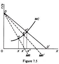
So long as the price-discriminating monopolist manages to reap part of the consumers surplus his total revenue and his total profits will be higher, even if he sells the quantity 0X, which is defined by the intersection of his MC with his (Original) aggregate MR curve.
However, the quantity that the discriminating monopolist supplies will be higher than OX if he can charge more than two prices in various sectors of the market, and his total revenue will be higher still.
The increase in output is due to the gradual shift of the MR curve upwards and the consequent change of the point of its intersection with the given MC curve.
The shift of the MR curve, given that DD’ does not change, is due to the fact that the MR (at all levels of output) is higher when price discrimination is being adopted, because the lower price at which the new marginal unit is sold is not the same as for all previously sold units, which have been sold at higher prices via individual negotiations with the buyers. In figure 7.5, if P were uniform, the monopolist would sell 0X amount of output.
If price discrimination is applied, only the additional units are sold at gradually lower prices, and hence the MR shifts to the position MR’. The new equilibrium position is defined by Ɛ’, at which the quantity is 0X’ > 0X. In the limiting case of perfect discrimination the MR will coincide with the DD’ curve, since each unit is sold at its own price, the highest price that the buyers are willing to pay on a ‘take-it- or-leave-it’ basis. The equilibrium will be at Ɛ”, the output will be 0X” and the following condition will hold and the seller will have achieved the maximum increase in his revenue, reaping all consumers’ surplus.
MC = MR = AR = P
Mathematical derivation of the equilibrium position of the price-discriminating monopolist
Given the total demand of the monopolist
ADVERTISEMENTS:
P = f(X)
Assume that the demand curves of the segmented markets are
P, = f1(X1) and P2 = f2(X2)
The cost of the firm is
ADVERTISEMENTS:
C = f (X) = f (X1 + X2)


