Monopoly Equilibrium of a Firm in the Long Run | Markets

In this article we will discuss about the monopoly equilibrium of a firm in the long run.

The Long-Run Adjustment Process in a Single-Plant Monopoly:

In short-run equilibrium of a monopolistic firm, we know that the firm may earn more than normal or only normal profit, or, it may earn even less than normal profit, i.e., it may run into losses. Now if the firm is among the losses in the short run, then in the long run, it would want to move to such a position by changing the size of its plant that would enable it to earn at least the normal profit.

Again, if the firm earns only the normal profit or more than normal profit in the short run, then in the long run, it would want to move, by changing its plant size, to a position where it could earn a higher amount of profit.

Now, if the firm is not able to earn even the normal profit in the short run, and even in the long run, it cannot earn even the normal profit by changing its plant size, then it would be forced to leave the industry in the long run.

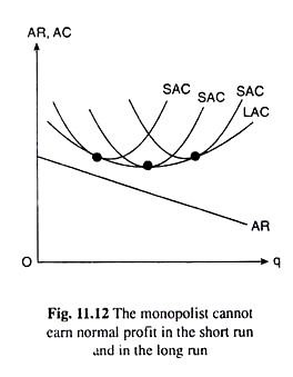
In Fig. 11.12, we see that the AR curve of the firm lies through­out its length below its LAC curve. In this case, in the short run and in the long run, the firm would have SAC ≥ LAC > AR at each level of output, i.e., here, by no means the firm can avoid a loss- making situation. Under the circumstances, the firm would leave the industry.

On the other hand, if even a portion of the AR curve of the firm lies above the LAC curve, then even if the firm incurs losses in the short run, it would be able to earn more than normal profit in the long run by suitably changing its plant size.

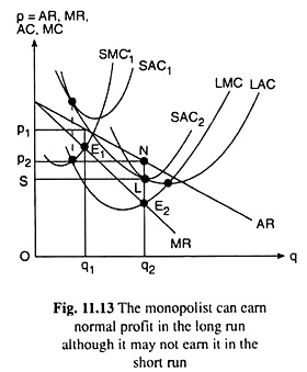
For example, in Fig. 11.13, if the firm’s short-run average and marginal cost curves are SAC₁ and SMC₁, then the firm would incur losses in the short run, because the whole of the SAC₁ curve lies above the AR curve. Here, in order to minimise the loss, the firm will produce the output of q₁ at the MR = SMC point, E₁ provided at q = q₁, the firm finds AR = p > AVC. The price of the product here would be p₁.

In Fig. 11.13, the firm would be able to earn positive economic profit (AR > LAC) in the long run. In order to maximise the level of profit, the firm would have to produce an output = q₂ at the MR = LMC point, E₂, according to FOC for maximum profit.

For achieving this, the firm would have to increase its plant size from SAQ to SAC₂. The second order condition for profit maximisation has also been satisfied at the point E₂, since here the LMC curve has intersected the MR curve from below, and then gone above it.

Therefore, here the point E₂ is the long-run equilibrium point of the firm. In Fig. 11.13, the firm has AR > LAC at q = q₂ and here it is able to earn a positive economic profit by producing and selling the output q = q₂ at the price p = p₂. The total amount of economic profit here is equal to □ p₂NLS.

Similarly, if in the short run, the firm earns the normal profit or more, then with a view to earning the maximum long-run profit, it would produce such an amount of output by changing its plant size that MR may become equal to LMC and the SOC for maximum profit is also satisfied.

A Monopolist cannot Earn More than Normal Profit in the Long Run:

If a purely monopolistic firm earns more than normal profit in the short run, then in the long run also, he will continue to do so, because by definition new firms cannot enter the monopolistic industry in the long run, and so there would be no sharing of profits, or, competition among the firms.

However, some economists are of the opinion that whatever may be the nature of the market organisation, competitive or monopolistic, no firm whatsoever would be able to earn more than normal profit in the long run. In other words, a monopolistic firm also, like a competitive firm, would be able to earn just the normal profit in the long run.

According to these economists, if the “ingredients” that are responsible for the monopolistic character of the organisation are capitalized, then the total cost of production would increase to such an extent that the eco­nomic profit of the monopolist will be reduced to zero.

We may explain the point with the help of an exam­ple. Let us suppose that the monopolist sells mineral water and this water is available from a particular spring. The monopolistic character of the business arises from the ownership of the land on which this spring is situ­ated.

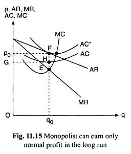
Let us suppose that the AR and AC curves shown in Fig. 11.15 are the average revenue and average cost curves of the monopolistic firm. On the basis of these curves, we obtain that the maximum profit price-output combination of the firm is (p₀, q₀), which is obtained at the MR = MC point E.

Here the amount of economic profit of the firm would be

π = TR – TC

= □ Op₀Fq₀ – □ OGHq₀

= □ p₀FHG

Since this profit emerges from the unique character of the land due to the existence of the spring on it, it should be considered while estimating the value of the land. In other words, if the monopolist wanted to sell the land, its price should reflect the profit which is equal to □ P₀FHG in our example.

In fact, as a result of competition among the potential customers of the land, its price will be increasing till it becomes so high that the profit estimated after taking into account the price of the land should fall to zero.

The flow of economic profit would be positive so long as the price of the land does not reach the said high ‘level’ and, so long as the price remains below that level, it would increase under the pressure of competition.

Now, even if the present owner of the land, i.e., the monopolistic seller of the mineral water, does not sell the land, he would include the cost of holding the land, i.e., the interest on the potential value of the land, in the fixed costs of his business. Consequently, in Fig. 11.15, the average cost (AC) curve of the firm would shift to a higher level from AC to AC*.

However, his MC curve’s position would remain unaffected, since an increase in total fixed cost cannot influence the MC. Therefore, the point of intersection E of the MR and MC curves would remain the same and, therefore, equilibrium output of the monopolist would remain unchanged at q₀, but his economic profit would reduce to zero.

In Fig. 11.15 we see that when the average cost curve of the monopolist is AC*, AR has been equal to AC at q = q₀ which implies AR x q₀ = AC x q₀ => TR = TC, i.e., the amount of economic profit of the monopolist has been obtained to be π = TR – TC = 0. Let us see why. At q = q₀, the firm has MR = MC, i.e., at q = q₀, the TR and TC curves have touched each other, and so, at q = q₀, the AR and AC curves also would touch each other.

Therefore, at the output level of q = q₀, the monopolist’s long-run economic profit would be equal to zero.

Therefore, in the above analysis, we arrive at the conclusion that, like the competitive firm, the monopolistic firm also would not be able to earn more than normal profit in the long run.