Monopoly in a Perfectly Competitive Market (With Diagram)

Let us make an in-depth study of the monopoly in a perfectly competitive market.

Monopoly:

A monopolist is a sole producer of a product.

If the monopolist decides to raise the price of the product, he need not worry about competitors.

The monopolist is the market and has complete control over the amount of output offered for sale. But this does not mean that the monopolist can charge whatever price he wants — at least if his aim is to maximise profit.

To maximise profit, he must first determine the market demand and its cost which is crucial for a firm’s decision-making. Given this knowledge, he must then decide how much to produce and sell. The price the monopolist charges then follows directly from the market demand curve.

Marginal Revenue and Average Revenue:

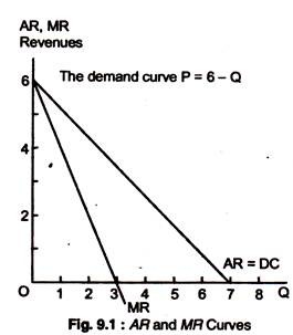
The monopolist needs to know the marginal revenue (MR) in order to choose his profit maximising output level. The average revenge curve of the monopolist is just the market demand. To get the relationship among total, average and marginal revenue, consider a firm facing the following demand curve P = 6 – Q.

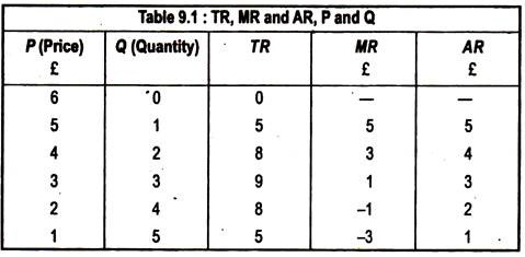
Table 9.1 shows the relation of total, average and marginal revenues. Note that revenue is zero when the price is £6, because, at this price nothing is produced and sold. However, at a price £5, one unit is sold, and the revenue is £5.

As quantity increases from 1 to 2, revenue increases from £5 to £8 and the MR is £3 and so on as the table shows. When MR is positive, revenue is increasing with quantity, but when MR is negative, revenue is decreasing with quantity.

When the demand curve is downward- sloping, the price (AR) > MR because all units must be sold at the same price. To increase sales, the price must fall. Table 9.1 shows TR, MR and AR.

Fig. 9.1 plots AR and MR curves for the data in Table 9.1. Demand curve is a straight line; in this case MR curve has twice the slope of the demand curve.

Output Decision of a Monopolist:

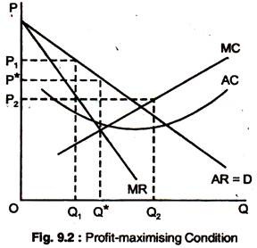
What quantity should the monopolist produce? If the objective of the monopolist is to maximise profit, a firm must produce output where MC = MR. This is the solution to the monopolist’s problem. In Fig. 9.2, the market demand curve, D, is the average revenue curve which specifies the price per unit that the monopolist receives as a function of its output level.

Also shown are MR, AR and MC curves and ACC. MR = MC at Q* output level and from the demand curve, we find the price P* that corresponds to this quantity Q* which is the profit-maximising quantity, because, a smaller output Q₁ receives higher price P₁. As Fig. 9.2 shows, MR > MC at output Q₁.

Thus, if the monopolist produces a little more than Q₁ he would receive extra profit and thereby increase his total profit. The monopolist could keep increasing output, adding more to his profit until output Q*, at which the incremental profit earned from producing one more unit is zero.

So, the small output Q₁ is not profit- maximising, even though it allows the monopolist to charge a higher price. By producing Q₁ instead of Q* the monopolist would reduce his total profit.

The larger quantity Q₂ is, likewise, not profit-maximising. At this point MC > MR, thus, if the monopolist produces a little less than Q₂, he would increase his total profit. The monopolist could increase his profit even more by reducing output to Q*.

Algebraically also, we can see that Q* maximises profit. Profit π is the difference between TR and TC, both of which depend on Q.

π(Q) = TR( Q) -TC( Q).

As O is increased from zero, profit will increase until it reaches a maximum, and then begin to decrease. Thus, profit-maximising output is such that the incremental profit resulting from a small increase in Q is zero (i.e. dπ-dQ = 0). Then,

dπ/dQ = dTR/dQ – dC/dQ = 0; where, dTR/dQ =MR and dC/dQ = MC, so the profit- maximising condition is that MR – MC = 0, or MR = MC.

Example:

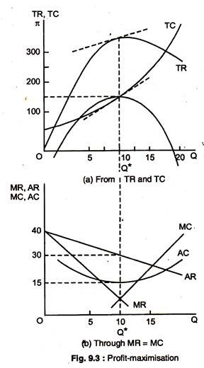
To understand this result clearly, let us look at an example. Suppose the cost of production is TC(Q) = 50 + Q², where, 50 is a fixed cost, and Q² is the variable cost.

And, suppose, demand is given by P(Q) = 40 – Q. By equating MR and MC, we can verify that profit is maximised when Q = 10, which corresponds to a price of £30. [AC is ( TC(Q)/Q=50/Q +Q ) and MC is dC/dQ = 2Q. TR (Q) = P(Q)Q = 40Q – Q². so, MR = 40 – 2Q. Equating MR = MC gives 40 – 2Q = 2Q or Q = 10. Substituting Q in demand equation: P(Q) = 40-10 .^.. P = 30 ]

TC, TR and π are plotted in Fig. 9.3(a). When the firm produces no output or little output, profit is negative because of the fixed cost. Profit increases with output, until it reaches a maximum of £150 at Q* = 10, and then decreases as Q is increased further.

And, at the point of maximum profit, the slopes of the TR and TC curves are the same. The slope of the TR curve dTR/dQ, or MR, and the slope of the total cost curve is dTC/dQ or MC. Profit is maximised when MR = MC, so the slopes are equal.

Fig. 9.3(b) shows the corresponding AR and MR curves, and AC and MC curves, MR = MC at output level Q* = 10. At this quantity, AC is £15 per unit, and P is £30 per unit, so average profit is £30 – £15 per unit. Since 10 units are sold, profit is (10)(15) = £150.

A Rule of Thumb for Pricing:

We know that price and output should be chosen so that MR = MC, but how does the manager of a firm find the correct price and output level, in practice? Managers may have only limited knowledge of the AR and MR that their firms face.

Similarly, they might have little knowledge about the firm’s MC curve. Thus, we want to translate the condition that MR should equal MC into a rule of thumb that can be more easily applied in practice.

To do this, we write the expression MR = dR/dQ = d (PQ)/Q

It may be noted that the extra revenue from an incremental unit of quantity, d(PQ)/dQ, has two components. Producing one extra unit of output and selling at price P brings in revenue of (1)(P) = P. Since the firm faces a downward-sloping demand curve, producing and selling an extra unit also results in a small drop in price dP/dQ, which reduces the revenue from all units sold. Thus, MR = Q dP/dQ =P+P (p/Q)(dP/dQ)

We find the expression on the right by taking the term Q(dP/dQ) and multiplying and dividing it by P. The elasticity of demand is defined as E_d = (P/Q) (dP/dQ). Hence, (Q/P)(dP/ dQ) is reciprocal of the elasticity of demand, 1/E_d, measured at the profit-maximising output, and MR = P + P(1/E_d).

Now, since the objective of the firm is to maximise profit, we can equate MR = MC: P + P (1/E_d) – MC, which can be rearranged to give us

P-MC/P = 1 /E_d………….(1)

This provides a rule of thumb for pricing. The term P-MC/P  is the markup over MC as a percentage of price which states that this mark-up should equal minus the inverse of the elasticity of demand.

Equivalently, we can rearrange this as:

P = MC/1+(1/E_d)

For example, if the elasticity of demand is -4 and MC – £9 per unit,

P = £ 9 /(1-1/4) = £ 9×4/3 = £12 per unit.

How does the price fixed by a monopolist compare with the price under competition? In a perfectly competitive market, as we know, P = MC. A monopolist charges a price that exceeds MC, by an amount that depends inversely on the elasticity of demand.

As the mark up equation (1) shows, if the demand is extremely elastic, E_d is a large negative number, and P will be very close to MC, so the monopolised market looks much like a competitive one. In fact, when demand is very elastic, there is very little benefit to being a monopolist.

Shifts in Demand:

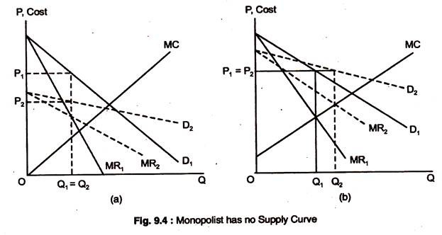
In a competitive market, there is a relationship between price and the quantity supplied. That relationship is the supply curve which tells us how much will be produced at every price. A monopolist has no supply curve. There is no one-to-one relationship between price and the quantity supplied.

The reason is that the monopolist’s output decision depends not only on the MC, but also on the shape of the demand curve. As a result, shifts in demand do not trace out a series of prices and quantities, as happens in a competitive market. Instead, shift in demand may lead to changes in price with no change in output, changes in output with no change in price, or changes in both.

Fig. 9.4(a) and 9.4(b) show this. In Fig. 9.4, the demand curve is initially D₁, the corresponding MR curve is MR₁, and the monopolist’s initial price and quantity are P₁ and Q₁. In Fig. 9.4(a) the demand curve shifted down and related the new demand and MR curves are shown as D₂ and MR₂. The MR₂ intersects the MC curve at the same point as MR₁ does. As a result, the quantity produced remains unchanged but the price falls to P₂.

In Fig. 9.4(b) the demand curve is shifted up. The new MR curve, MR₂, intersects the MC curve at a larger quantity Q₂. But the shift in the demand curve is such that the price charged is the same. Shifts in demand usually cause changes in both quantity and price.

But the case shown in Fig. 9.4 illustrates an important distinction between competitive supply and monopoly. In the case of a competitive industry, a specific quantity is supplied at each price. No such relationship exists for a monopolist.

Measuring Monopoly Power:

The distinction between a perfectly competitive firm and a monopoly is that, for the competitive firm, P = MC, for the firm with monopoly power, P > MC.

Thus, a natural way to measure monopoly power is to examine the extent to which the profit-maximising P > MC. We can, in fact, use the mark up ratio of (P-MC)/P that was introduced as a rule of thumb pricing.

This measure is introduced by Lerner and is called Lemer’s Degree of Monopoly Power: . L=  (P-MC)/P.This Lerner Index has always a value of zero and one. For a perfectly competitive firm, L = 0, so that P = MC. The larger is L, the greater the degree of monopoly power.

This index of monopoly power can also be expressed in terms of the elasticity of demand facing the firm. Using equation (1), we know that

L = (P-MC)/P = 1/E_d ………..(3)

Where E_d is the elasticity of the firm’s demand curve, and not the market demand curve. If the elasticity of demand for the firm is -6, the degree of monopoly power is 1/6. It may be noted that considerable monopoly power does not necessarily imply high profits. Profit depends on AC relative to price.

Rule of Thumb of Pricing and Elasticity of Demand:

We have already seen how the relationship among price, MC, and the elasticity of demand can be used as a rule of thumb for pricing by a monopolist.

Equation (2) allowed us to compute price as simple mark up over MC:

P = MC/1 + (1/E_d)

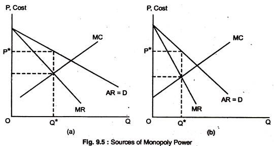
This provides a rule of thumb for any firm with monopoly power, if we remember that E_d is the elasticity of demand for the firm and not the industry. If the demand is elastic as in Fig. 9.5(a), the mark up is small, and the firm has little monopoly power. If the firm’s elasticity of demand is small, the mark-up will be large. Fig. 9.5(a) and 9.5(b) illustrate these two cases.

Some firms have considerable monopoly power, and other firms have little or none and it is the monopoly power which determines firm’s ability to set price > MC, and the amount by which P > MC depends inversely on the firm’s elasticity of demand. The less elastic its demand curve, the more monopoly power a firm has. The ultimate determinant of monopoly power is, therefore, the firm’s elasticity of demand.

Three factors determine a firm’s elasticity of demand. First, the elasticity of market demand. Second, the number of firms in the market. Third, the interaction among firms.

Let us examine each of these three determinants of monopoly power.

Elasticity of Market Demand:

The demand curve of a pure monopolist is the market demand curve. In this case, the firm’s degree of monopoly power depends on the elasticity of market demand. More often, several firms compete with one another, and then the elasticity of market demand sets a lower limit on the elasticity of demand for each firm.

The demand for oil is fairly inelastic, at least in the short-run — that is why OPEC could raise oil prices far above the MC during the 1970s and 1980s. The demand for other commodities — such as tea, cocoa, coffee and copper — are much more elastic, this is the reason why attempts by producers to cartelize those markets and raise prices have, largely, failed.

In each case, the elasticity of market demand limits the potential monopoly power of individual producers.

Number of Firms:

The number of firms in the market also limits the monopoly power of a firm. Other things being equal, the monopoly power of each firm will fall as the number of firms increases. As more firms compete with each other, each firm will find it difficult to raise prices and avoid losing sales to other firms.

What matters is not mainly the number of firms, but the number of “major players.” For example, if only two or three firms account for 85 to 90% of sales in a market, with another 30 firms accounting for the remaining 10 to 15%, the two or three large firms might have considerable monopoly power because the market is highly concentrated.

The greatest fear of some business is competition. This is, mainly, true, because if there are only a few firms in a market, their managers would prefer that no new firms enter the market. An increase in the number of firms can reduce the monopoly power of each incumbent firm and, so, their competitive strategy is to create barriers to entry.

Sometimes there are natural barriers to entry, because of the patent on the technology needed to produce a particular product. Other legally created barriers to entry is a copyright granted to a particular firm, and the need for a government license can prevent new firms from entering the market and so on.

Finally, economies of scale may make it costly for more than a few firms to supply the entire market. In some cases the economies of scale could be so large that it is most efficient for a single firm — a natural monopoly — to supply the whole market.

Interaction among Firms:

Sometimes interactions among the competing firms is an important determinant of monopoly power. Suppose there are three firms in a market who are aggressively competing with each other to capture more market share. This might drive price to a nearly competitive level. Each firm might be afraid to raise its price for fear of losing market to its competitors.

On the other hand, the firms might not compete much. They might collude. At the extreme, they might form a cartel and, thereby, agree to limit output and raise prices. Raising prices together, rather than individually, is more profitable, so collusion would generate substantial monopoly power.

Here we want to point out that other things being equal, monopoly power is small when firms compete and is large when they cooperate.

Moreover, monopoly power often changes over time, as its behaviour, its operating conditions, and the behaviour of its competitors, change. Thus, monopoly power must be thought of in a dynamic context.

For example, the market demand curve may be highly inelastic in the short-run but much more elastic in the long-run. Monopoly power in the short-run can make an industry more competitive in the long-run. Large short-run profits can attract new firms to enter the industry, thus, reducing monopoly power over the long-run.

Social Cost of Monopoly:

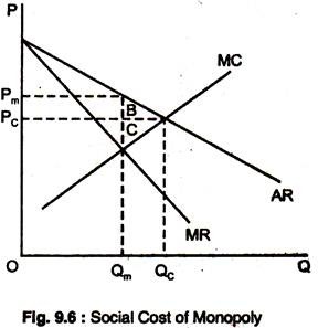
In a competitive market, P = MC, while, in a monopoly market, P > MC. Since monopoly power results in higher prices and lower quantities, we would expect it to make consumers worse-off and producers better-off. Suppose we value the welfare of consumers and producers in the same way.

Does monopoly power make consumers and producers in the aggregate better or worse-off? The area A +B + C shows changes in consumers’ and producers’ surplus when moving from competitive price and quantity, P_C, and Q_C, respectively, to a monopolists price and quantity, P_m and Q_m, respectively.

Under monopoly the price is higher, and consumers buy less and those consumers who buy the good lose surplus of an amount given by the area A. Those consumers who could not buy because of higher price, P_m, of the good also lose consumers’ surplus, represented by the area B. Because of the higher price, total loss of consumers’ surplus is the area A + B.

The producer gains area A at the higher price but loses area C. The total gain in producers’ surplus is A – C. Subtracting the loss of consumers’ surplus from the gain in producers’ surplus, we see a net loss of surplus represented by B + C.

This is the deadweight loss from monopoly power which is the social cost of inefficiency. There are two ways to limit monopoly power and thus, to eliminate inefficiency — Natural Monopoly was nationalize in Europe and Regulated in the USA.

Natural Monopoly: Public or Private:

First, we discuss industries in which scale economies are large, competition may not be feasible or it may sacrifice scale economies to an extent that competition is undesirable. Before 1980, such industries were thought to require so much regulation that they might as well be state owned.

Nationalization is the acquisition of private companies by the public sector.

After 1980, the UK & New Zealand pioneered a programme of privatization, now emulated by many other countries.

Privatization is the return of state enterprises to private ownership and control.

In some industries like utilities such as telecommunications, gas, water, etc. more extensive regulation was needed whenever international competition is not vigorous.

Natural Monopoly:

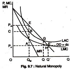
Fig. 9.7 shows an industry with steadily falling LAC as output rises. Only one private firm can survive in such an industry. Any firm that expands output can cut costs and undercut its rivals. Facing a d c DD & MR, the resulting monopolist produces QM and earns profits PMCBE.

The efficient point is E’ where LMC = DC = MBC. A private monopolist sets MC = MR, produce QM & earns profits PMCBE. The deadweight loss under private monopoly is AEE’. If by law monopolist was forced to charge a price P_c, the monopolist would face a horizontal dc P_cE up to the output Q’.

Since P_C would then also be MR, the monopolist would produce at E’ where the MR = MC (coincide). Although efficient, society cannot face the monopolist to produce here in the long-run. Since £”lies below LAC the monopolist is making losses and would rather go out of business.

A natural monopoly’s AC* keep falling as its output rises. It undercuts all smaller competitors. At this output the SMB. P_m > SMC at A. The monopolist makes too little. SMB = SMC at the output Q’ and the efficient point for society is E’.

The private monopoly creates a deadweight burden AEE’. You sit on the Competition Commission (CC) investigating the monopolist. If you split up the firm, a lot of small firms each producing at a higher AC, a waste of resources.

You can order the firm to produce at the efficient point E’, with desired output Q’, but the price P_c < AC at Q’. It makes losses. Since MC < AC when AC is falling, forcing a natural monopolist to price at mc is always loss making. You cannot force a private firm to make losses. It will then shut down.

One solution is a regulatory body, such as OFTEL that regulates BT. It aims to get close to the efficient allocation E’ while letting the monopolist to break-even after allowing a proper deduction for all economic costs. By making the monopolist produce Q at P = AC at this output, the deadweight burden is cut from AEE’ to GHE’.

An even better solution is to allow the monopolist to charge a two-part tariff. A two-part tariff charges a fixed sum for access to the service & then a price per unit that reflects the MC of production.

A two-part tariff uses fixed charges to pay for fixed costs, and marginal charges to cover MC. In Fig. 9.7 the monopolist is told to charge P. for each unit of the good consumer demand the socially efficient output Q Since the monopolist is a price-taker at the controlled price P_c, it is loss-minimising for the monopolist to produce Q at which P = MR = MC. The regulator then allows the monopolist to buy the minimum fixed charge necessary to ensure that it breaks even after allowing for all relevant economic costs.

A third solution to monopoly problem is to order the monopolist to produce at the efficient point E’ at the price P_c and provide a government subsidy to cover the losses. It is socially desirable to make the efficient output Q’ in the cost-minimising way. If the subsidy solution is adopted, there is pressure for the government to get involved in running the industry so that operations can be carefully monitored.

Three problems recur with all these solutions to the problem of natural monopoly. First, information is costly for monitors to acquire. It is hard to ensure the industry does minimise costs. Unnecessarily high costs can be passed on under AC pricing (Solution 1), a result in a higher fixed charge to ensure break-even under a two-part tariff (Solution 2), or can require a larger subsidy (Solution 3).

In each case the regulatory body has the difficult task of trying to make the N. M. as efficient as possible. (N. M. = Natural Monopoly).

The second problem is regulatory capture (R. C.). R. C. implies that the regulator gradually comes to identify with the interest of the firm it regulates, becoming its champion not its watchdog. The regulated firms devote considerable time, effort and money to lobbying the regulator.

More subtly, the regulated firm has all the inside information about its own activities, information that the regulator needs to acquire. Regulators build up contacts with the regulated. Eventually, the regulator can sympathies with the problems of the regulated.

Third, regulators find it hard to make credible commitments about their future behaviour. For example, the regulator may encourage the monopolist to invest by promising ‘high’ regulation in the future.

Once the investment is made and a cost sunk, the regulator then faces the temptations to change the ground rules, toughening requirements. Foreseeing this, the monopolist never invests and there is problem of underinvestment. During post-war period, (1950-1980) many European governments concluded that the least bad solution was nationalization.