Price-Output Determination in a Multi-Plant Monopoly

In this article we will discuss about the price-output determination in a multi-plant monopoly in the long run.

In the long run, a monopoly organisation with a number of plants may increase (or decrease) the number of its plants with a view to obtain the profit-maximising solution. Now, each plant of the monopolist may be of a different size, and in the long run the size of each plant is a variable.

However, in the long run since all sorts of input adjustments are possible, the LAC curve and the associated SAC curves of each plant of the monopolist would be identical, for what is good for a particular plant is good for every other plant. The size of each plant should be such as would enable the firm to produce the same quantity of output at the same minimum possible (average) cost.

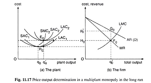
That is, in the long run the monopolist will select the minimum point on the identical LAC curve of each plant, which is also the minimum point of the associated SAC curve. This point would be like the point R₀ in Fig. 11.17 (a).

At this point, the quantity of output to be produced at each plant is q₀ and the minimum long-run average cost of production at q = q₀ would be R₀q₀—this is also the minimum possible average cost in the long run of his total output of all the plants taken together.

In the long run, as the number of plants of the multi-plant monopolist increases so that a larger quantity of output may be produced, the SAC curves along with their envelope LAC curve in each plant will shift upwards, as it has done from the lower LAC to the higher LAC curve in Fig. 11.17(a) and, therefore, the minimum possible average cost in the long run will also rise.

This is because, in order to produce a larger quantity of output, the firm would be willing to purchase the inputs in larger quantities and, consequently, the prices of these inputs will rise.

It is clear from the above discussion that as the multi-plant monopolist increases his output by setting up additional plants in the long run, his minimum possible LAC at each plant will increase, as it has increased from R₀q₀ to E₀ q’₀ in Fig. 11.17(a).

That is, along with an increase in his total output, there would be a rise in LAC which implies (owing to the average-marginal relation) that his LMC also would rise (and LMC would be greater than LAC), i.e., his LMC curve would slope upward towards right.

In Fig. 11.17(b), we have drawn such an LMC curve of the firm and also its AR (demand) and MR curves. Here, the point of intersection of the MR and LMC curves, F₀, is the firm’s long-run equilibrium point. At this point, the firm’s MR and LMC both have been equal to F₀q₀* and its total long-run equilibrium output has been obtained to be q₁, and this output can be sold in the market at the price of p₀*.

It may be remembered that the LAC = F₀q* is equal to the SMC and LMC of each plant [shown in Fig. 11.17 (a)] at the minimum point of a plant LAC curve, which has been here LAC₂. In Fig. 11.17, at the firm’s LMC = F₀q₀* = E₀q₀‘, the quantity produced in each of its plants is q = q₀‘. Here, the number of plants of the firm would be q₀*/q’₀ = n (say).

Since the price, or average revenue of the total output, and, therefore, of the output of each plant is p*₀ and the long-run average cost of the output of each plant and of the total output is E₀q’₀ = F₀q₀* = OH₀, the average amount of profit per unit of output is p*₀ – OH₀ = p*₀H₀ and the total amount of profit of the monopolist here would be equal to p*₀H₀ x q*₀ = □ p*₀H₀F₀G₀.