The reason for a monopolist (or any other firm) to apply price discrimination is to obtain an increase in his total revenue and his profits.
By selling the quantity defined by the equation of his MC and his MR at different prices the monopolist releases a higher total revenue and hence higher profits as compared with the revenue he would receive by charging a uniform price.
We will start from the simplest case of a monopolist who sells his product at two different prices.
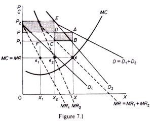
It is assumed that the monopolist will sell his product in two segregated markets, each of them having a demand curve with different elasticity. In figure 7.1 the demand curve D1 has a higher price elasticity than D2 at any given price. The total-demand curve D is found by the horizontal summation of D1 and D2. The aggregate marginal revenue (MR) is the horizontal summation of the marginal-revenue curves MR1 and MR2. The marginal-cost curve is depicted by the curve MC.
ADVERTISEMENTS:
The price-discriminating monopolist has to decide:
(a) The total output that he must produce,
(b) How much to sell in each market and at what price, so as to maximize his profits.
The total quantity to be produced is defined by the point of intersection of the MC and the aggregate MR curves of the monopolist. In figure 7.1 the two curves intersect at point ε, thus defining a total output 0X which must be produced. If the monopolist were to charge a uniform price this would be P, and his total revenue would be 0XAP.
His profit would be the difference between this revenue and the cost for producing OX. However, the monopolist can achieve a higher profit by charging different prices in the two markets. The price and the quantity in each market is defined in such a way as to maximize profit in each market.
Thus in each market he must equate the marginal revenue with the MC. However, the marginal cost is the same for the whole quantity produced, irrespective of the market in which it is going to be sold. The marginal revenue in each market differs due to the difference in the elasticity of the two demand curves.
The profit in each market is maximized by equating MC to the corresponding MR:
MR1 = MC
ADVERTISEMENTS:
In the first market profit is maximized when
MR2 = MC
Clearly the total profit is maximized when the monopolist equates the common MC to the individual revenues
MC = MR1 = MR2
If MR in one market were larger, the monopolist would sell more in that market and less in the other, until the above condition was fulfilled. Graphically the determination of the prices and quantities in the two markets is defined as follows.
From the equilibrium point e we draw a line perpendicular to the price axis. This line cuts the marginal revenue MR1 at point Ɛ1 and the marginal revenue MR2 at point Ɛ2. Clearly at these points we have the required equality
MC = MR1 = MR2
From Ɛ1 and Ɛ2 we drop vertical lines to the quantity axis, and we extend them upwards until they meet the demand curves D1 and D2 respectively. These vertical lines define the output and price in each market. Thus in the first market the monopolist will sell 0X1 at a price P1, and in the second market the monopolist will sell 0X2 at the price P2.
Clearly 0A1 + 0X2 = 0X.
ADVERTISEMENTS:
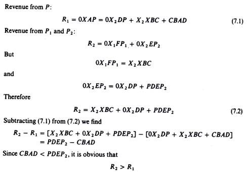
From figure 7.1 it is obvious that the total revenue from price discrimination is larger than the revenue 0XAP which would be received by charging a uniform price P. With price discrimination the total revenue is
Comparing this revenue with the revenue from the unique price P we find the following:
Note that PDEP2 is the additional revenue from selling 0X2 at price P2 which is higher than P, while CBAD is the loss in revenue from selling 0X1 at price P1 which is lower than P. The additional revenue from selling 0X2 at a higher price more than offsets the loss of revenue from selling 0X2 at a lower price, so that total revenue from price discrimination is larger. Since the cost of producing 0X is the same irrespective of the price at which it will be sold, the profits from price discrimination are larger as compared with those that would be obtained from selling all the output at the uniform price P.
ADVERTISEMENTS:
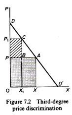
The above case has been called third-degree price discrimination by the British economist Pigou. The increase in total revenue is achieved by taking away part of the consumers’ surplus. To understand this let us concentrate on the demand curve, D (figure 7.2). If the monopolist sold all 0X at P he would receive 0XAP, and the consumers would have a surplus of PAD. Assume now that the monopolist sells 0X1 at the price P1 and the remaining quantity X1X at the price P. His total revenue will be that is, the monopolist has managed to take the part PBCP1 from the consumers’ surplus.
0X1CP1 + X1XAB = 0XAP + PBCP1
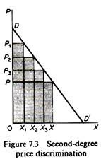
If the monopolist can negotiate and sell at more than two prices (higher than P), for example to sell 0X1 at P1, X1X2 at P2,X2X3 at P3 and X3X at P, he will receive a still larger part of the consumers’ surplus (figure 7.3). This is called a second-degree price discrimination.
ADVERTISEMENTS:
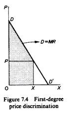
In the limiting case in which the monopolist can negotiate individually with each buyer and sell each unit of output at its corresponding price as shown from the DD’ curve, then he will receive the entire consumers’ surplus (figure 7.4). This is known as first-degree price discrimination or as take-it-or-leave-it’ price discrimination, because in negotiating with each buyer the monopolist charges him the maximum price he is willing to pay under threat of denying the selling of any quantity to him: he offers each buyer a ‘take-it-or-leave-it’ choice. In this case the demand curve also becomes the MR curve of the monopolist.
