Aggregate Supply and Demand (With Diagram)

Read this article to learn about the Aggregate Supply and Demand which is explained with the help of diagrams!

1. Reason, 2. Result,  3. Impact and 4. Conclusion!

 

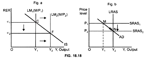
Short run equilibrium point → M (Fig. 18.18)

Reason:

Price level is fixed (P₁)

Due to lack of effective demand (AD), economy produces at less than full employment level (Y₁)

As AD < SAS (SAS – short run aggregate supply)

Price falls from P₁ to P₂

Result:

Supply of real balances (M/P) rises from M/P₁ to M/P₂

LM curve shifts to the right from LM₁ to LM₂ (Fig. 18.18a)

Impact:

RER falls from є₁ to є₂

NX rises, income level rises from Y₁ to Y₂ and the economy reaches full employment level (Y₂), that is, at point N (Fig b).

Conclusion:

On comparing a fiscal expansion under flexible rates with the results we derived for fixed rates we find that under fixed rates fiscal expansion is highly effective in raising the equilibrium output but under flexible rates fiscal expansion does not change the equilibrium output, there is full crowding out.