8 Main Effects of Change in Investment

The following points highlight the eight main effects of changes in investments. The effects are: 1. A Change in Desired Investment 2. The Income-Expenditure Approach 3. The Leakages-Injections Approach 4. Non-Autonomous Investment 5. A Change in Desired Consumption and Saving 6. The Paradox of Thrift 7. Induced Investment and Thrift 8. Inflationary and Deflationary Gaps.

Effect # 1. A Change in Desired Investment:

Suppose there is an increase in the amount of investment expenditure of business firms. Business firms may be desirous of investing more if, for exam­ple, there occurs a technological change in a major industry such as the electronics industry. If a new product (say VCR) is invented firms may decide to build new plants in order to serve the growing market for the product.

The effect of an increase in planned investment on the equilibrium level of income may be shown by using any of the two approaches to the theory of in­come determination, viz., the income-expenditure ap­proach or the leakages-injections approach.

Effect # 2. The Income-Expenditure Approach:

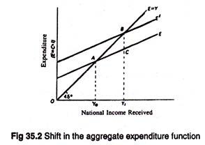
If there is an increase in planned investment ex­penditure the aggregate expenditure (E = C + I) curve shifts upward. This indicates that society is planning to spend more at each level of income. As a result national income rises. This is shown in Fig. 35.2. Here the initial expenditure function is E, and the initial equilibrium level of income is Y₀.

If planned investment increases, the aggregate expenditure cur­ve would shift to the left. Since investment is au­tonomous and hence independent of income there is a parallel shift of the investment function (not shown here) and thus in aggregate expenditure function from E to E’.

As a result equilibrium income rises to Y₁. This is quite obvious: if desired spending on the na­tion’s output rises, equilibrium national income rises, too.

The opposite type of change may also be shown in the diagram. If autonomous investment falls equi­librium national income will also fall. Thus the ba­sic point to note is that any act of autonomous spend­ing (such as investment expenditure) will have an income-creating effect.

Effect # 3. The Leakages-Injections Approach:

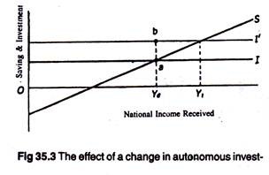
In Fig. 35.3 the original saving and investment schedules are S and I. They intersect at point a to gen­erate an equilibrium national income Y₀. Now we let the investment schedule to shift upward to I’.

This implies that at the same equilibrium level of income Y₀, total investment spending increases from aY₀ to bY₀. In other words, there is more desired investment at each level of income. As a result equilibrium income rises from Y₀ to Y₁.

Thus while a rise in planned investment expenditure raises equilibrium national income, a fall in planned in­vestment expenditure lowers it. Why do these happen? The reason is easy to find out.

When the saving curve remains unchanged, the upward shift of the investment curve implies that, at the initial level of income, Y₀, business firms (or investors in general) wish to inject more funds (money) into the circular flow by way of investment than households (or savers in general) wish to withdraw through savings.

So there is an excess or planned investment over planned saving as shown by the distance ab in Fig. 35.3.

This excess of injection over leakage creates ex­tra demand in the country for goods and services. So output (GNP) has to increase to meet the extra de­mand, consequently national income rises. If income increases, consumption and saving will both increase. The process of income generation will continue until and unless the additional saving is again equated to additional desired investment.

Two related points:

Two points may be noted in this context. Firstly, here we are dealing with con­tinuous flows measured per unit of time, i.e., flows in each period. Secondly, we are dealing with real flows, i.e., the quantities of consumption and capital (investment) goods people wish to purchase at differ­ent levels of real national income.

Effect # 4. Non-Autonomous Investment:

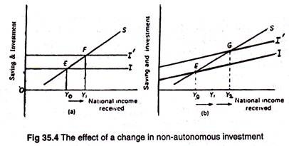
We may now drop the assumption that all in­vestment in autonomous. We may now suppose that investment were to increase with income. This would imply that an increase in investment would cause in­come to rise and this, in its turn, would cause the level of desired investment to increase. As a result there will be a further increase in national income.

In other words, if investment like consumption also depends on national income or its rate of change there will not only be secondary consumption spend­ing but secondary investment spending, too. This additional investment will lead to further increase in national income as is illustrated in Fig. 35.4.

In Fig. 35.4 (a) investment is autonomous, in which case a rise in investment causes the equilibrium level of in­come to rise from Y₀ to Y%. But if investment is non- autonomous as shown in Fig. 35.4 (b) a shift of same magnitude of the investment line would cause the equilibrium level of income to rise from Y₀ to Y₂.

Effect # 5. A Change in Desired Consumption and Saving:

We may now consider the effect of an upward shift in the consumption function or, what comes to the same thing, a downward shift of the saving func­tion.

Let us argue, for instance, that households in the aggregate decide to spend (save) Rs. 500,000 more (less) at each level of income. This will also have an ef­fect on the equilibrium level of national income. We may now discuss this point in detail in terms of the two approaches.

(1) The income-expenditure approach:

If con­sumption spending increases, the aggregate expendi­ture curve shifts upward to E’ as in Fig. 35.2. As a result equilibrium income rises from Y₀ to Y₁. The opposite effect will be produced if saving increases at each level of income or consumption expenditure falls, i.e., there is an upward (downward) shift in the saving (consumption) function and hence in the ag­gregate expenditure function.

(2) The leakages-injections approach:

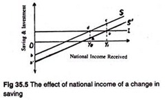
If house­holds plan to spend (save) more (less) at each level of income, the saving schedule will shift downward from S to S’ as in Fig. 35.5. This leads to a rise in national income from Y₀ to Y₁. Equilibrium is re­stored at point b because the desire of households to save less (shown by a downward shift of the saving schedule) causes national income to rise until desired saving falls to its original level (i.e., bY₁ = dY₀).

The converse is also true. An increase in planned sav­ing and a corresponding upward shift of the saving schedule will lower equilibrium income from its orig­inal level. This can also be shown diagrammatically. So we have observed that a rise (fall) in consumption spending, which is the same thing as a fall (rise) in planned saving, raises (lowers) equilibrium national income.

Effect # 6. The Paradox of Thrift:

It is often observed that what is good for an individual (or from the micro point of view) is not necessarily good for the society (or from the macro-point of view). When, for instance, an individual attempts to save more it is good for him.

Thrift at the individual level may lead to wealth and prosperity, while dissaving may lead to ultimate bankruptcy. But if all individuals become desirous of saving more at the same time the result may be dis­astrous. There may be a fall in the actual saving of the community. This peculiar result is known as the paradox of thrift or the paradox of saving.

We have observed that if the saving curve shifts to the left there is a fall in national income. Suppose S’ is the original saving curve in Fig. 35.5. It now shifts to the left to S. The increase in thriftiness will lead to a fall in the equilibrium level of national income from Y₁ to Y₀.

This point has been explained by R. G. Lipsey and C. Harbury in the following words: “The upward shift in the saving schedule causes planned saving to exceed planned investment at the initial equilibrium level of income. National income falls and this in­duces a decline in planned saving. Income continues to fall until saving is again equal to investment.”

However, we are assuming here that investment is autonomous. Here a fixed level of investment takes place at all levels of income. This has an important implication for the theory of income determination.

In this case saving has to fall back to the original level so that it is again equated to the original level of in­vestment. Thus, attempts to save more are frustrated due to income fall. And income continues to fall un­til everyone ends up saving exactly what they were saving before income change.

The opposite situation is one of a decrease in the thriftiness or an increase in planned consumption spending. This will cause a downward shift of the saving function—e.g., from S to S’ in Fig. 35.5.

Due to increased desire to save on the part of households, desired leakages will be less than desired injections at the initial level of national income—Y₀ in Fig. 35.5. This will cause national income to rise. The income expansion process will continue until the actual vol­ume of saving is again equated to its initial level but at a new, higher level of national income.

The validity of the paradox:

The paradox is valid only when we make the following two assumptions:

1. Firstly, we have to assume that actual (na­tional) income is below its full employment level. Thus unused (idle) productive capacity will permit the economy to increase its GNP whenever aggregate demand increases.

The converse is also true: any­thing that reduces aggregate demand will lead to a fall in output and employment. This results follows from the fact that in Keynesian income and employ­ment model national income is demand determined.

Thus, anything which reduces aggregate effective de­mand such as an increased desire to save lowers em­ployment, output and income.

2. Our second assumption is that saving and investment plans are taken independently. So, ac­cording to Keynes’ theory, there is no reason why the amount that business firms plan to invest at any level of income should be related to the amount that house­holds plan to save.If any of the two assumptions do not hold, the paradox will not be encountered.

1. For instance, the first assumption may be in­correct if actual income is already equal to potential (full employment) income. In this case a fall in desired saving of the household (or an increase in household consumption expenditure) will not lead to an increase in real output and employment. The reason is simple; the economy has already reached the point of maxi­mum output, i.e., its full employment point.

In such situations, an increase in consumption spending will cause inflation. On the other hand, an increase in sav­ing, on a decrease in consumption, with its accompa­nying decrease in aggregate spending, will tend to reduce output and employment by creating a defla­tionary gap in the economy.

2. If the second assumption appears to be wrong, the paradox of thrift will not hold. Let us argue, for example, that the saving and investment functions are inter-linked because changes in household saving cause changes in investment. In this case, whenever, the is a change in the desire to save, there could be an off-setting shift in the investment function.

If the two plans are inter-linked the following consequence is likely to follow: An increased desire to save would shift the saving function upward. But, it would per­mit more investment and therefore, would also shift the investment function upward. As a result of these two off-setting shifts, no downward pressure on na­tional income would be created.

Keynes, however, noted that saving and invest­ment decisions are taken largely by different groups in society—by households and business firms, respec­tively. It may apparently seem that there is no mech­anism by which a change in the amount that house­holds plan to save at a fixed level of income will cause a change in the amount that business firms plan to in­vest at the same level of income.

However, in practice we find a possible mecha­nism that tends to exert some influence on both saving and investment decisions. Thus, for the paradox of thrift to hold we have to argue that interest rates do not adjust automatically so as to bring about an equal­ity between planned saving and planned investment at each and every level of national income (as has been postulated by the classical economists.)

Prediction:

A close look reveals that the paradox of thrift is not a paradox in the true sense. Instead it is a straight forward prediction that follows logically from the theory of income determination. The para­dox gives us the following important insight: sudden shifts in consumption spending and saving do exert expansionary and constractionary demand pressures on the economy in the short run by affecting aggre­gate demand.

However, growth theorists believe that supply conditions are more important (than demand conditions) in determining total output. Therefore, it is incorrect to say that a fall in planned saving will increase national income in the long term.

Effect # 7. Induced Investment and Thrift:

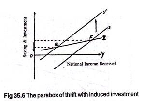
The paradox can be developed further if we as­sume that investment is non-autonomous or induced. We now argue that investment increases with income. So that investment line now slopes upward (with pos­itive rather than zero slope).

The slope of the line mea­sures the marginal propensity to invest which is ex­pressed as i = ∆I_p/∆Y. Here ∆I_p is the absolute change in induced private investment and ∆Y is the abso­lute change in national income.

In Fig. 35.6 we again consider the effect of an upward shift of the saving schedule. This figure explains the paradox fully in the sense that “not only does increased saving bring about a lower level of income and investment but it also leads, ultimately, to less being saved.”

This ef­fect is produced because there is lesser ability to save at lower levels of national income. People’s plan (or, desire) to save more has been frustrated by the fall in income which a fall in saving causes.

The paradox can be stated as follows:

An increased desire to save may lead to a fall in the actual saving of the community: (This sim­ply means that sometimes the cure is worse than the disease.) Keynes also pointed out that the effect of increa­sed thriftiness also depends upon the state of the econ­omy.

During inflation an increase in thriftiness or a decrease in consumption expenditure is desirable be­cause it may act as an anti-inflationary measure by eliminating excess demand.

If, on the other hand, the economy suffers from deep depression, with wide­spread unemployment, the increase in thriftiness could be quite disastrous. It would take the economy into a cumulative (vicious) deflationary spiral.

Thus, if planners and policy-makers attempt to ‘tighten our belts’ during depression, the problem is likely to be more serious. In other words, the depression is likely to be made even worse. As J. M. Keynes rightly com­mented: “when-ever you save five shillings you put a man out of work for a day.”

Effect # 8. Inflationary and Deflationary Gaps:

We have already referred to the potential output of an economy. Actual output may deviate from the full employment or potential output. It is defined as that level of income which, if attained, is just sufficient to keep all resources fully employed at any particular time.

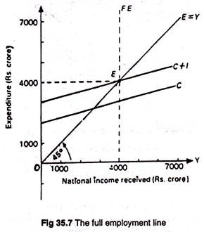
In Fig. 35.7 this represented by the vertical line, FE, which may be called the full employment line. In this diagram the equilibrium level of national income (Rs. 4000 crores) corresponds to the full employment level. It may, however, be noted the equilibrium level of national income is not necessarily the full employ­ment level.

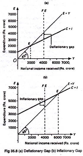
If there is deficiency of effective demand (C +1) in the economy the equilibrium will occur at a lower level of income and to the left of the FE line. This is illustrated in Fig. 35.8 (a). Here we observed that ac­tual income is Rs. 2000 crores in equilibrium. There is therefore severe unemployment in the economy.

De­mand deficiency is measured by the distance between the 45° line and the C + I line at the full employ­ment level of national income. This vertical distance is known as the deflationary gap.

In order to eliminate unemployment or to enable the economy reach full employment, it is essential to shift the C + I line up­ward by Rs. 1000 crores.An exactly opposite type of situation is shown in Fig. 35.8 (b). In this diagram equilibrium level of national appears to the right of the FE line at Rs. 6000 crores.

This type of situation is likely to occur when people are trying to buy more goods and ser­vices than can be produced by the way of utilizing all its resources.

There is full-employment, and there is “too much money chasing too few goods.” This excess demand pressure pulls up prices. The excess demand for goods and services is being met in money, and not in real, terms. The vertical distance between the C + I line and the 45° line at full employment measures what Keynes calls the inflationary gap.

In Keynes’ model, for demand-pull inflation to occur, there must exist such a gap in the economy. In this case it would be necessary to lower the C + I line by Rs. 1000 crores to eliminate excess demand pres­sure and hence inflation. Of course, their are other causes of inflation also.