Determination of Equilibrium National Income Determined in a 4-Sector Economy

We know that by exporting goods, a coun­try can expand its market overseas, while by importing goods it reduces the market for domestic goods abroad.

Anyway, aggregate demand becomes C + I + G + (X – M). The difference between X and M is referred to as balance of trade.

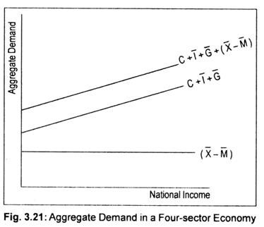
For convenience, we assume that, like investment and government expenditures, X and M are autonomous or independent of the level of income. This is shown in Fig. 3.21 where (X – M ) line shows autonomous net exports. C + I + G line is the aggregate expenditure of a closed economy. If we add net exports to this aggregate expenditure line, we get aggregate expenditure of an open economy, i.e., four-sector model.

There are again two alternative appro­aches to determine equilibrium national income in a four-sector model.

First approach states that equilibrium national income must equate the aggregate demand, i.e.,

Y = C + I + G + (X – M)

Alternative equilibrium condition states that sum of all savings, taxes and import must equal the sum of all investment expenditure, government expenditure and export, i.e.,

S + T + M = I + G + X

(i) Determination of Equilibrium National Income when C + I + G + (X – M) Line Cuts the 45° Line:

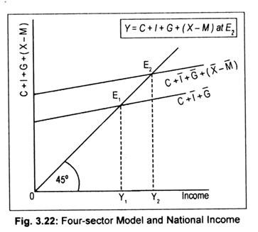
In a four-sector economy, equilibrium national income is determined when aggregate demand equals aggregate supply. This means that when C + 1 + G + (X – M) line cuts the 45° line, equilibrium national income is determined. E₁ in Fig. 3.22 is the equilibrium point when the economy does neither export nor import.

If exports and imports are taken into account C + I + G line will shift to C + I + G + (X – M). This aggregate expenditure line now cuts the 45° line at point E₂. Corresponding to this equilibrium point, equilibrium national income, thus, determined is OY₂. Thus, (positive) net exports results in an increase in national income and negative exports (i.e., M > X) results in a reduction in national income.

(ii) Equilibrium National Income at the Intersection of. S + T + M and I + G + X Line:

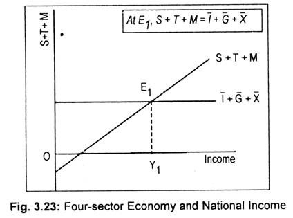
Equilibrium national income is determined when the sum of S + T + M equals the sum of 1 + G + X. In Fig. 3.23, I + G + X line has been drawn as parallel to the horizontal axis since these three elements are assumed to be autonomously determined. On the other hand, since saving, tax and import are assumed to be the direct functions of income, S + T + M line has been drawn as an upward rising line. As these two curves intersect each other at point E₁, equilibrium national income, thus, determined is OY₁.