Determination of Equilibrium National Income in a Two-Sector Economy!

1. Meaning of Equilibrium:

By equilibrium we mean the state of balance or state of no change. By equilibrium national income we refer to that level of national income which remains unchanged at a particular level.

At the equilibrium level of national income there is no tendency for income/output to rise or fall.

In the Keynesian two-sector economy there are only household and business sectors.

Government is absent and the economy is a closed one. In this simple economy, there are two elements of national income—consum­ption and investment, i.e., C + I. An economy is said to be in equilibrium when aggregate expenditure equals aggregate income or aggregate money value of all goods and services.

Aggregate demand is, thus, sum of consumption demand and investment demand. Since, in a two-sector economy, there are only two goods—consumption goods and investment goods—aggregate expenditure is, the sum of consumption and investment expenditures. Thus, aggregate demand (C + I) equals aggregate expenditure (C + I).

Alternatively, whenever aggregate income equals aggregate expenditure, leakages from and injections into the circular flow of income become equal to each other. In a two-sector economy, saving is the only source of withdrawal and investment is the only source of injection. Thus, an economy is said to be in equilibrium when saving (i.e., withdrawal) equals investment (i.e., injection).

The above argument, thus, suggests that there are two alternative approaches of national income determination. First approach slates that the equilibrium level of national income is determined by the equality of aggregate demand (or aggregate expenditure) and aggregate supply of output. In terms of a diagram, one can say that in a two-sector economy, the equilibrium level of national income is determined at that point where C + I line cuts the 45° line. This approach is, thus, known as income-expenditure approach or aggregate demand-supply approach.

Aggregate demand = money value of output (income)

or Y = C + I …(3.17)

Alternative approach states that, when injection (I) equals leakage (S) in a two-sector economy, equilibrium level of national income is determined. In terms of a diagram, when saving line and investment line intersect each other, equilibrium level of income is determined.

Leakage (saving) = injection (investment)

or S = I …(3.18)

Remember that these two approaches are alternative to each other.

2. Methods to Determine Equilibrium National Income:

Now these approaches will be explained in detail:

(i) First Method: Aggregate Income- Expenditure Approach:

In a two-sector Keynesian model, aggregate demand is composed of planned or desired consumption demand and planned investment demand. The total of planned expenditure (C + I) must be equal to the value of output or income for a simple economy to be in equilibrium. Or when the C + I line cuts the 45° line, an equilibrium level of income is determined. In other words, an equilibrium level of national income is determined at that point where aggregate demand (C + I) equals aggregate supply (i.e., the country’s aggregate output or national income).

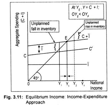
To illustrate equilibrium national output graphically, we use Fig. 3.11 where we measure national income on the horizontal axis and aggregate demand or spending (C +1) on the vertical axis. The 45° line is purely a reference line; any point on this line is equidistant from both the horizontal and vertical axes. Aggregate spending (C + I) is equal to the value of income or output on this 45° line. For our exposition purposes, this line can be thought of as an aggregate supply curve, though it is not a ‘true’ aggregate supply curve.

With no government and foreign trade sectors, aggregate demand/expenditure is the sum of consumption demand and investment demand. In Fig. 3.11, CC’ is the planned consumption line. It shows the level of consumption for each level of income. Investment expenditure is assumed to be autonomous. To demonstrate this, investment line 1 has been drawn parallel to the horizontal axis.

By summing up the consumption and autonomous investment schedules one obtains aggregate demand schedule (C + I). The vertical distance between the CC’ line and the C + I line measures the volume of autonomous investment. Point E is the equilibrium point since C + I line cuts the 45° line at that point. Equilibrium level of income, thus determined, is OY_E since it is the only level of income at which aggregate demand and aggregate value of output (or income) are equal to each other.

We can show that this equilibrium level of income is a stable one. This means that if the level of income is either more than or less than OY_E then there will be a tendency for the level of income to move toward OY_E. Otherwise, equilibrium is said to be unstable. Suppose, if income is OY, (< OY_E), aggregate demand will exceed aggregate supply or aggregate output. Now there will be an excess demand for goods and services, resulting in an unplanned reduc­tion of inventories. (Remember that invento­ries are part of investment.) As inventories decline, business firms step up production.

Thus, output will continue to rise till OY_E is achieved. Similarly, at OY, level of income, aggregate supply exceeds aggregate demand. This means an excess supply of goods and services. People are not willing to purchase all the goods that the nation has produced. Thus, there will be an unintended accumula­tion of inventories by producers. Firms will now be forced to cut back production. Output will continue to decline till OY_E is attained. Only at OY_E there is neither unplanned accu­mulation nor depletion of inventories. Thus, OY_E is stable equilibrium national income.

To have a stable equilibrium of income one condition is needed—slope of the line C + I must be equal to the slope of the CC’ line. The slope of the consumption line CC’ is the MPC whose value must always be less than unity. Diagrammatically, this means that the C + I line must cut the 45° line from above. If C + I line cuts the 45° line from below then the value of MPC would be greater than unity and equilibrium income, thus, determined in this manner would be unstable.

(ii) Alternative Method: Saving-Investment Approach:

Total withdrawals from and injections into the circular flow determine equilibrium national income. In a two-sector economy, withdrawal comprises only saving while injection comprises only investment. Equilibrium national income is determined at that point when planned saving and planned investment are equal to each other. Diagram­matically, at the intersection of the saving and investment line, equilibrium national income is determined.

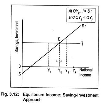
In Fig. 3.12, we measure national income on the horizontal axis and savings and investment on the vertical axis. SS’ is the planned saving curve which has a negative intercept in the sense that at low level of income since consumption exceeds income savings must be negative. As usual, I is the autonomous investment line drawn parallel to the horizontal axis. As SS’ curve cuts I at point E, equilibrium level of income is thus determined at OY_E. In other words, planned saving and planned investment are equal only at the intersection of the two curves and, thus, equilibrium income is OY_E. And this equilibrium income is a stable one.

To see whether OY_E is a stable equilibrium income, we consider OY₁ or OY₂ level of income. If the deviation from OY_E level of income gets corrected or if the equilibrium income OY_E is attained after deviation, then equilibrium is said to be a stable one. At OY₁ level of income, investment (injection) exceeds saving (leakage). Aggregate demand must exceed aggregate output. This will result in an unplanned reduction of inventories to meet excess demand. Consequently, output will rise until planned saving and planned investment are equal.

Similarly, at OY₂ level of income, since saving exceeds investment, aggregate demand falls short of aggregate supply. Hence, an excess supply of commodities will appear leading to an unplanned accumulation of inventories. This will act as an incentive to cut back output. Output will continue to decline until point E is reached where OY_E equilibrium level of national income is determined. Thus, OY_£ is a stable equilibrium.

The condition for stability is that the saving curve must be positively sloped. MPS is the slope of the saving function. To have stability, the value of MPS must be positive but less than one. Remember that MPS is complementary to MPC. If MPC < 1, then MPS must be less than one since MPC + MPS = 1. Thus, the condition for stability in equilibrium income in both the approaches is the same, i.e., 0 < MPC < 1.

A Numerical Example on the Determination of Equilibrium National Income in. a two-sector economy:

Suppose, consumption (C) is given by the consumption function

C = 5 + 0.8Y

where Y is income.

Assume that investment is autonomous (I) and is given by

I = Rs. 10

With this information, we want to derive the equilibrium values of income, consumption, saving and investment.

Solution:

Equilibrium condition is Y = C + I, where C = a + bY and I = I. Putting the values of C and I, we obtain

Y = a + bY + I

or Y – bY = a + I

or Y (I – b) = a + I

Y = 1/1-b (a + I)

Here, Y is the equilibrium level of income. Substituting the consumption and investment equations into equation Y, we get 1

Y =1/1-0.8 (5 + 10) – Rs. 75

Thus, C = 5 + 0.8(75) = Rs. 65, and

S = Y-C = 75 – 65 = Rs. 10

I = Rs. 10

The above approach has an alternative approach, known as saving-investment approach.

Alternative solution:

Equilibrium condi­tion now is S = I

S = Y – C = Y – a – bY

= – a + (1 – b) Y

Assuming 1=1, the equilibrium condition becomes

-a + (l-b) Y = I

So the equilibrium level of income is

Y= 1/1-b (a + I)

From the consumption function C = 5 + 0.8Y we find the values of a and (1 – b). If a = 5 then (-a) = -5, and if b = .8 then (1 – b) = 0.2. Now putting these values into saving and investment equation, we get

– 5 + 0.2Y = 10

0.2Y-5 = 10

0.2Y = 10 + 5

or Y = 15/0.2 = Rs. 75

If Y = Rs. 75, saving must be equal to Rs. 10 since consumption is Rs. 65.

Note that, since the two forms of equilibrium condition are equivalent, the level of income must be the same.

Practise 1:

C = Rs. 10+0.6Y, I = Rs. 12 crore. Find equilibrium I, C and S, where Y, C and S have the usual meanings.

Ans:

Y = Rs. 55 crore, C = Rs. 43 crore, and S = Rs. 12 crore.

Practise 2:

Suppose S = -Rs. 40 + 0.20Y and I = Rs. 60. Find the equilibrium income, saving and consumption.

Ans:

Y = Rs. 500, S = Rs. 60

C = Rs. 440

3. Equilibrium Income is not Necessa­rily Full Employment Income:

We have demonstrated how equilibrium level of national income in the Keynesian framework is determined. But this equilibrium income must not necessarily be full employment income (designated as Y_F in Figs. 3.11 and 3.12). Equilibrium income determined (OY_E) is definitely less than full employment income (OY_F). This means that aggregate demand (C + I) is inadequate to maintain full employment. At the full employment level, aggregate output becomes maximum.

But, in the Keynesian system, aggregate demand or aggregate spending creates an income level which is necessarily less than full employment income. This equilibrium income has been described by Keynes as ‘underemployment equilibrium’. To reach ‘full employment equilibrium’, Keynes prescribed a fiscal policy measure which aims at stepping up government expenditure and tax cuts.