Determination of National Income by the Three-Sector Economy

Let us Learn about the Determination of National Income by the Three-Sector Economy.

An economy without government spending or taxation is hardly conceivable today. To make our analysis a realistic one, we assume the existence of the government sector that has the power to spend and collect taxes. In a two-sector economy, GNP = C + I.

But in a three-sector economy, without any trading relationship with the outside world, GNP = C + I + G. Thus, government spending is an important element of aggregate demand or expenditure. Similarly, imposition of taxes by the government results in a change in disposable income. With the inclusion of taxes in our present analysis, national income becomes

Y = C + S + T

However, basic equilibrium condition in this complicated economy does not change: Aggregate demand (C + I + G) must equal the aggregate output, i.e.,

Y = C + I + G

Alternative equilibrium condition states the equality between leakages and injections, i.e.,

S + T = I + G

If the government does not impose any taxes (i.e., T = 0) to finance its expenditure programme, the equilibrium condition becomes

S = I + G

(a) Determination of Equilibrium Income when C + I + G Line Cuts the 45° Line:

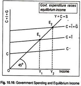
In a three-sector economy with government spending and zero taxes, equilibrium national income is determined when aggregate supply equals aggregate demand. That is to say, equilibrium national income is determined at that point when C + I + G line cuts the 45° line (Fig. 10.16).

To explain this, let us assume that, like private investment, government spending is also autonomous. This means that G is independent of the level of income. CC’ is the consumption function. If autonomous investment of I is added to this consumption line we obtain C + I line. This aggregate private demand (C + I) schedule cuts the 45° line at E_t and the corresponding equilibrium level of income is OY₁.

Now, by adding autonomous public expenditure to private demand, we obtain the aggregate demand function C+I+G. This schedule cuts the 45° line at E₂. The new equilibrium level of income is OY₂. Thus, an injection of government spending results in an increase in income and employment.

(b) Equilibrium Income at the Intersection of S and I + G Line:

For equilibrium, toted leakages must equal total injections. As we assume that our govern­ment spends only but does not collect taxes, total leakages now constitute only saving. However, private investment and public investment are injected here in the circular flow of income.

Thus, equilibrium condition can be written as:

S = I + G

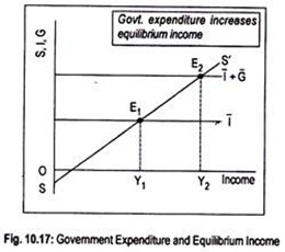
It is assumed here that both private investment and government spending are autonomous. To represent this, we have drawn investment line T parallel to the horizontal axis in Fig. 10.17. If autonomous government spending is added we obtain the line I + G.

The distance between land I + G line represents the volume of public investment. SS’ and I intersect each other at E₁ and the equilibrium level of income is OY₁. Now, an increase in government expenditure has the same effect on aggregate demand and income as an increase in autonomous private investment. I + G line now cuts the saving line SS’ at E₂.

Since government expenditure represents an addition to aggregate demand, equilibrium level of income rises to OY₂, greater than the original income OY₁. Thus, an increase in government expenditure results in an increase in equilibrium level of income.