Determination of National Income: Keynes’s Two Sector Model

Let us make in-depth study of Keynes’s two sector model in relation to determination of national income.

Keynes’s Income-Expenditure Approach:

Keynesian theory is relevant in the context of the short run only since the stock of capital, techniques of production, efficiency of la­bour, the size of population, forms of business organisation have been assumed to remain constant in this theory.

Further in his model of income determination Keynes assumed that price level in the economy remains unchanged.

Therefore, in the Keynesian theory which deals with the short run, the level of income of the country will change as a result of changes in the level of labour em­ployment.

Thus, in an a free market economy in the short run, when capital stock and technology remain unchanged, income is a function of labour employment. In fact, both income and employ­ment go together. The higher the level of employment, the higher the level of income. As level of employment is determined by aggregate demand and aggregate supply, the level of income is also determined by aggregate demand and aggregate supply.

The, aggregate expenditure shows aggregate demand for goods and services. Keynesian theory of income determination can be explained by assuming two sectors in the economy, namely, households and business firms Keynes focused on this simply two sector model of determination of national income and derived conclusions regarding policy formulation from this basic model.

Analysis of determination of national income can be extended to incorporate Government and foreign trade. We start with the analysis of determination of national income by taking a simple two-sector economy with a fixed price level. The two sectors are consumption demand by households and investment demand by entrepreneurs.

Aggregate Expenditure:

Aggregate expenditure is the total expenditure which at given fixed prices all households and business firms want to make on goods and services in a period at various levels of national income. In Keynes’s original model aggregate expenditure is in fact aggregate demand at given prices.

In a two-sector closed economy, aggregate expenditure or aggregate demand consists of two components:

First, there is consumption demand, and secondly, there is a demand for capital goods, which is called investment demand. Thus, by aggregate expenditure we mean how much expenditure ‘the households and the entrepreneurs are willing to make on consumption and investment. Therefore,

Aggregate Expenditure = Consumption Demand + Investment Demand

AE = C + I

where AE stands for aggregate demand, C for consumption demand and I for investment demand. Note that aggregate demand implies aggregate expenditure (AE), consumption demand (C) implies consumption expenditure and investment demand (I) implies investment expenditure. Thus

AE=C +1

Consumption Demand:

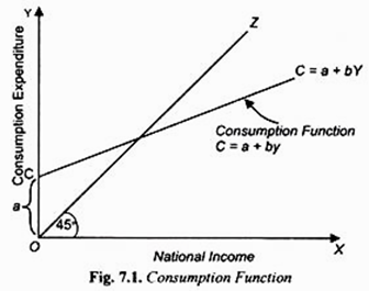
As for consumption demand, it depends upon the propensity to consume of the community and the level of national income. Given the propensity to consume, as income increases, consumption demand will also increase. In other words, given the propensity to consume, consumption demand is a function of income. Consumption function can take several forms. The most common form of short-run consumption function is

C = a + bY

where a is the intercept term of the function and represents autonomous consumption whereas b represents the slope of the consumption function.

Consider Fig. 7.1 in which national income is measured along the X-axis and consump­tion demand (C) is shown on the Y-axis. In this figure, a straight line OZ which makes 45° angle with the X-axis has been drawn. This straight line OZ with 45° angle with the X-axis represents the reference income line to measure the difference between consumption and level of income.

This is also often called income line. This 45° line represents national income in money terms. In fact, national product and income are the same things. In this figure a curve C has also been drawn which repre­sents consumption function, C = a + by of the community.

This curve of consumption function slopes upward from left to right, which shows that as income increases the amount of consumption demand also increases. As income line OZ makes 45° angle with the X-axis, the gap between the consumption function curve C and the income line OZ represents the saving of the community.

The reason for this is that a part of the income is consumed and a part is saved, i.e., National Income = Consumption + Saving. This is also written as Y = C + S, where y represents income, C consumption and S saving. It will be seen from Fig. 7.1 that the gap between the consumption function curve C and the income line OZ goes on increasing as income increases. In other words, the amount of saving or saving gap increases as income increases.

It is worth mentioning that in the short-run consumption function does not change. This is because the propensity to consume, that is, the whole consumption function curve C depends upon the tastes, preferences, the income distribution in the society, the population level, wealth of the people etc., which do not undergo much change in the short run. The implication of the stability of consumption function is that the consumption demand is primarily determined by the level of current national income.

However, through changes in monetary policy and fiscal policy by the Government the consump­tion function can be shifted. For example, when rate of interest, an instrument of monetary policy, is reduced, the people borrow more for durable consumer goods such as cars, air conditioners, houses and with this at a given level of income consumption demand increases causing upward shift in the consumption function curve.

Similarly, when income tax, an instrument of fiscal policy, is reduced disposable income of the households increases and as a result at a given level of national income (GDP), consumption demand increases leading to the upward shift in consumption function.

Investment Demand:

The other component of the aggregate demand is invest­ment which is a crucial factor in the determination of equilibrium le el of national income.

Investment demand depends upon two factors:

(1) Marginal efficiency of capital and

(2) Rate of interest.

Of these two factors, rate of interest is comparatively stable and does not frequently change in the short run. Therefore, the fluctuations in the level of investment demand chiefly depend upon the changes in the marginal efficiency of capital. The marginal efficiency of capital means the expected rate of profit which the business community hopes to get from the investment in capital assets.

Marginal efficiency of capital depends upon the replacement cost of the capital goods on the one hand, and profit expectations of entrepreneurs on the other. Profit expectations are more important because they often change even in the short run and cause fluctuations in investment. If the level of national income and employment is desired to be raised in a free market capitalist economy, then steps should be taken which will raise the expectations of the entrepreneurs (i.e., business firms) regarding profit-earning from investment.

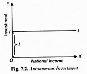
In any particular year, there will be a given level of invest­ment demand which, as seen above, is determined by marginal efficiency of capital and a given rate of interest. However, in Keynes’s theory investment being determined by marginal efficiency of capital and rate of interest does not depend on the level of income.

Thus, in Keynesian theory of income determination, investment does not vary with change in income. In other words, in Keynes’s directly income-expenditure analysis investment is treated as autonomous of income that is investment does not change with a change in the level of income.

This type of investment is shown in Figure 7.2. In actual practice when the level of income rises, the demand for goods will also rise and this will favourably affect the expectations of the entrepreneurs regarding making of profits. Rise in the profit expectations will raise the marginal efficiency of capital which in turn will increase the level of investment.

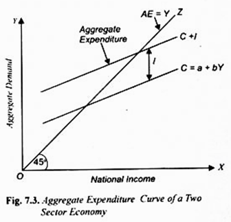
But it is quite clear that investment demand does not directly depend upon income; it is only affected indirectly by changes in income. Therefore, in our Figure 7.3 we have taken a given amount of investment demand independent of the level of income and added it to upward sloping consumption function curve to get aggregate expenditure curve C + I. The distance between the C curve and the C + I curve is parallel to the C curve throughout which indicates that the level of investment is constant and does not change with the change in income.

It may however be noted that with either a change in the rate of interest or in margin­al efficiency of capital investment will change. Therefore, in income-expenditure diagram as shown in Fig. 7.3, a different new amount of investment of will have to be taken.

Aggregate Output:

In the short run the level of national income and employment in a free-market economy depends upon the equi­librium between aggregate expenditure and aggregate output. We have also explained above the various components of aggregate expenditure on goods and services. We now run to explain the aggregate supply and factors on which it depends. It is important to note again that Keynes in his analysis assumed that prices and wages remain constant in the short run.

In an economy without any role of Government, national income means the total money value of final goods and services produced in an economy in a year.

There are two important constituents of aggregate output:

1. The supply or output of final consumer goods and services in a year; and

2. The output of capital goods in a year which are also called producer goods because they help in producing further goods. Net addition to the stock of capital goods in a year is called investment.

National income is the same thing as national product as both represents the value of output of final goods and services produced. In fact, aggregate supply or money value of national product of goods and services is distributed among the various factors of production as wages, rent, interest and profits as rewards them for their contribution to the national product.

The aggregate output which is also sometimes referred to as aggregate supply of goods of an economy depends upon the stock of capital, the amount of labour used and the state of technology. In the short run, stock of capital remains constant and therefore output can be increased by increasing the amount of labour employed.

Like the classical economists Keynes also thought that aggregate output or national income depend the short-run production function with a given capital stock and constant technology.

Thus, we have the following production function in the short run:

Y = (N, K, f)

where Y is national output, k is the constant amount of capital stock, T is the constant state of technology and N is the labour employed which is a variable factor. It may be noted that the amount of production which a given amount of labour can produce depends upon the given stock of capital and state of technology.

The higher the level of technology, more can be produced with the help of given resources. Since J.M. Keynes in the nineteen thirties and we at present are concerned with the determination of income and employment in the short run, the stock of capital and the state of technology are assumed to be constant. For similar reasons, size of population is also assumed to be constant. However, the amount of labour employed out of this given size of population can vary depending upon the demand for labour.

45° Line as Aggregate Supply Curve of Output (With Fixed Price Level):

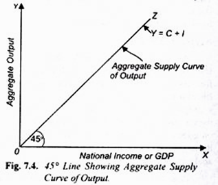
In Keynes’s income-expenditure analysis with which we are presently concerned we need to compare Gross Domestic Product (or National Income) with aggregate expenditure (AE), also called aggregate demand (AD), which is represented on the vertical axis. For this purpose we draw a 45° line from the origin which helps us to transfer Gross Domestic Product or real National Income (i.e. gross supply of output at constant prices) from the horizontal axis to the vertical axis for compar­ing it with total expenditure on goods and services.

At every point of this 45° line from the origin, the vertical distance equals horizontal distance which measures real national income or GDP which is generally denoted by Y. This 45° line is also called income line along which Y = C + S because income can either be consumed or saved.

The essential feature which emerges from all this is that more output will be pro­duced and supplied at the given price level in response to increase in aggregate demand or expenditure. In other words, whatever the ag­gregate demand, more output of goods will be produced and supplied at the same price before full-employment of resources is reached.

This type of aggregate supply curve has been shown by 45° OZ line drawn against the X and Y axes in Fig. 7.4 where along the X-axis real national income (GDP) and along the K-axis aggregate supply of output is measured. However, as noted above, aggregate output and real national income (GDP) are identical.

It follows from above that 45° line shows two things. First, it shows varying levels of aggregate production or the supply of goods (both consumer and capital goods) that will be offered for sale at the given price level at various levels of aggregate expenditure.

This shows that up to the level of full-employment of resources any amount of aggregate supply of output will be forthcoming at the given price level depending on the aggregate demand or expenditures. The greater the ag­gregate demand or expenditure, the greater the aggregate supply of output at the given price level. Secondly, it represents national income. In fact, as you would have read in national income accounting, national product and national income are the same things.

Equilibrium Level of National Income:

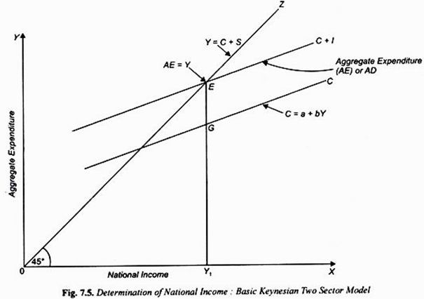
Now, we shall explain how through the intersection of aggregate demand and aggregate supply curves the equilibrium level of national income is determined in Keynes’s two sector model. C + I curve represents the aggregate expenditure and 45° OZ line represents aggregate supply of output.

Normally the goods and services are produced by firms when they think they can sell them in the market. There will be equilibrium in the goods market when total output of goods and services pro­duced will be equal to the total demand for output. Aggregate demand for them is represented by aggregate expenditure. In equilibrium aggregate expenditure (which is denoted by AE) must equal aggregate output (GDP).

Since aggregate output or GDP equals national income (K) we have the following condition for equilibrium:

AE = GDP = Y

It will be seen in Fig. 7.5 that aggregate expenditure curve (AE) or C + I curve intersects 45° line at point E which satisfies the equilibrium condition. That is, a point E which corresponds to the income level OY₁ aggregate expenditure is equal to aggregate output. Therefore, E is the equilibrium point and OY₁represents the equilibrium level of national income. Now, income cannot be in equilib­rium at levels smaller than OY₁ since aggregate expenditure exceeds aggregate supply of output as C + I curve which depicts aggregate expenditure of output lies above 45° line.

This excess demand will be met by the firms selling goods from their stocks or inventories of goods kept by them. This leads to the decline in inventories of goods below the desired levels. This unintended fall in invento­ries will induce the firms to expand their output of goods and services to meet the extra demand for them and keep their inventories of goods at the desired levels.

Thus when at a given level of national income, aggregate expenditure (i.e., aggregate demand) exceeds aggregate output, national income will increase. With this increase in national income or output, employment of labour will also rise to produce the increment in output. This process of expansion in output under the pressure of excess demand will continue till national income OY₁ is reached.

On the contrary, the equilibrium level of national income cannot be greater than OK, because at any level greater than OY₁ aggregate expenditure or demand (C + I) falls short of aggregate output. This will cause the increase in inventories of goods with the firms beyond the desired levels. To this situation of the unintended increase in inventories of goods, the firms will respond by cutting down production to keep their inventories at the desired levels.

Thus, deficiency in aggregate demand relative to the aggregate supply of output will lead to the fall in national income and output until the level OY₁ is reached where aggregate expenditure (C + I) is equal to the value of aggregate output. Thus, OY₁ is the equilibrium level of national income.

Principle of Effective Demand:

We have seen above that the equilibrium level of national income is determined by aggregate demand and aggregate supply of output. Consider Fig. 7.5 where it will be seen that, the prices remaining constant, aggregate expenditure (AE) curve C + I shows varying levels of aggregate expenditure at various levels of is not equal to aggregate output and there­fore determines the equilibrium national income is called effective demand.

In other words, effective demand is that level of aggregate demand (aggregate expenditure) which becomes effective in determining equilibrium level of income because it is equal to aggregate supply of output. This is called Keynesian principle of effective demand. In Fig. 7.5, the effective demand is equal to Y₁E. Note that the level of national income OY₁which has been determined, equals the effective demand Y₁E (OY₁ = Y₁E).

There are several other points on the aggregate expenditure curve but what distinguishes effective demand from all these points is that at this point aggregate expenditure is equal to aggregate output. On all other points aggregate demand is either more or less than aggregate output. Thus, the level of national income is determined by and equal to effective demand.

In a two sectors Keynesian model, we can express the principle of effective demand in symbolic terms as under:

Y = AE* = AD*

AE* = AD* = C + I

Y = AD* = C + I

where Y = National Income

AD* = Effective demand

C = Consumption demand

I = Investment

Note that star mark on AE or AD shows the aggregate demand which becomes effective.

Importance:

It is thus clear that national income and employment in the short run are deter­mined by effective demand or in other words, effective expenditure. The higher the level of effective demand, the greater the levels of national income and employment and vice-versa. Unemployment is due to deficiency of effective demand and the basic remedy to remove this unemployment is to raise the level of effective demand.

Due to their belief in Say’s law and in quick adjustment of wages and prices to balance between demand and supply the classical economists believed that effective demand was always large enough to ensure full-employment. But Keynes proved that it was not so and that is why the problem of involuntary unemployment was common in the free-market capitalist economies.

Equilibrium is not Necessary Established at Full-Employment Level:

The most important contention of J.M. Keynes in his now famous work “General Theory of Employment, Interest and Money” was that in a capitalist economy it is not necessary that the equilibrium level of income is established at the level of full-employment. This view of Keynes was quite contrary to the views of the classical economists who believed that the economy always tended towards full-employment. Keynes refuted this important idea of the classical economics.

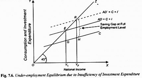
To understand the Keynesian viewpoint consider Fig. 7.6. Suppose the full-employment level of labour corresponds to the level of national income equal to OY_F. Thus represents the level of income at which there is full-employment in the economy. But, as seen above, the equilibrium level of income is not established at OY_F but at OY, at which some number of labour will be unemployed.

Thus equilibrium at OY_F is known as underemployment equilibrium. It is worth noting that in the situation depicted in Fig. 7.6 the equilibrium level of national income will be established at full-employment level only when investment demand is sufficiently large to fill the saving gap between income and consumption at the full-employment level of income OY_F.

It will be seen from Fig. 7.6, that corresponding to the full-employment level of income OY_F, RH is the saving of the community. Therefore, if the equilibrium is to be established at OK level, then investment demand must be equal to level of saving RH at full employment level of income Y_F.

But the prevailing investment demand is only equal to EG which is less than RH. With RH as the level of investment and the C curve as the level of propensity to consume, C + I curve intersects the 45° aggregate output curve OZ at point R and therefore determines equilibrium level of income equal to OY_F at which labour will be fully employed.

But there is no guarantee that the investment demand will be equal to the saving gap corresponding to full-employment level of income. There are various reasons for this. First, the people who save are not necessary those who make investment; while it is the general public which save but only few people constituting the entrepreneurial class undertakes investment. Secondly, the factors which determine saving are quite different from those which determine investment.

While the people save for providing for the education, marriages of their children and also for contingency purposes such as diseases and unemployment periods. They also save in order to acquire durable goods such as houses, gold and jewellery. They also save to accumulate sufficient funds for their old age.

But the level of investment depends upon marginal efficiency of capital and rate of interest in the short run and on the level of population, technological progress in the long run. Therefore, it is not essential that investment should be equal to the amount of savings by the people at full-employment level. If due to the adverse changes in the profit expectations of the entrepreneurs, level of investment falls, the equilibrium level of national income will also decline.

It is also worth noting that if aggregate expenditure increases beyond the C + I in Fig. 7.6 it will mean that the economy is spending and demanding more than it can produce. The result of this will be rise in prices of the commodities. In other words, if the investment demand in any year is higher than HR, then the inflationary process will start. In this situation, national income will rise beyond OY_F only in money terms but not in real terms.

Determination of Equilibrium Level of National Income: Algebraic Analysis:

A study of how the level of national income is determined will become more clear by using simple mathematics. As has been explained above, the level of national income is in equilibrium at which aggregate demand equals aggregate supply of output. In a simple model of income determination in which we do not consider the impact of Government expenditure and taxation and also exports and imports, the national income is the sum of consumption demand (C) and investment demand (I), that is,

Y = C + I

where Y stands for the level of national income.

Suppose the consumption function is of the following form:

C = a + bY

α is the intercept term in the consumption function and therefore represents the autonomous consumption expenditure which does not very with income, b is a constant which represents the marginal propensity to consume (mpc ∆C/∆Y). Thus total consumption demand is equal to the sum of autonomous consumption expenditure (α) and the induced consumption expenditure (bY).

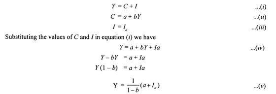
Now suppose that investment demand equals l_a. This investment I_a is autonomous because this does not depend on income. Thus, we get the following three equations for the determination of the equilibrium level of national income.

The equation (v) shows the equilibrium level of national income when aggregated expenditure equals aggregate supply of output. The equation (v) reveals that autonomous consumption and autonomous investment (a + I_a) generates so much expenditure or aggregate demand which is equal to the income generated by the production of goods and services.

From the equation (v) it also follows that the equilibrium level of national income can be known from multiplying the elements of autonomous expenditure (that is, a + I_a) by the term 1/1-b which is equal to the value of multiplier. Further, it also follows that equilibrium level of income is higher, the greater the marginal propensity to consume (i.e. b) and autonomous consumption (α) and autonomous investment (Iα).

Illustrations of Equilibrium Level of Income with Numerical Examples:

A few numerical examples will make it clear how the equilibrium level of national income is determined.

Problem1:

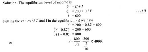
Suppose in an economy, autonomous investment (I) is Rs. 600 crores and the follow­ing consumption function is given:

C = 200 + 0.8K

Given the above, find out the equilibrium level of income.

Alternative Method:

In our algebraic analysis of equilibrium level of national income we have derived the following condition for equilibrium level of national income.

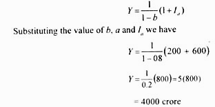
Y = 1/1-b (a+ I_a)

where 1/1-b is investment multiplier and b is marginal propensity to consume a is the intercept term in the consumption function. The above condition can also be used to determine the equilibrium level of national income. Marginal propensity to consume (b) in the given problem is 0.8 and the intercept term a equals 200. Using this alternative method we have

Problem 2:

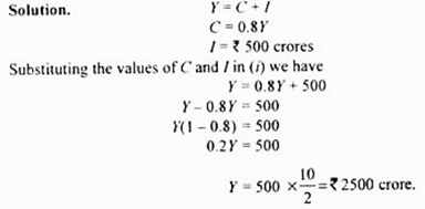
Suppose the consumption function of an economy is C = 0.8 Y. Planned investment by entrepreneurs for a year is Rs. 500 crores. Find out what will be the equilibrium level of income.

Problem 3:

For an economy following consumption function is given:

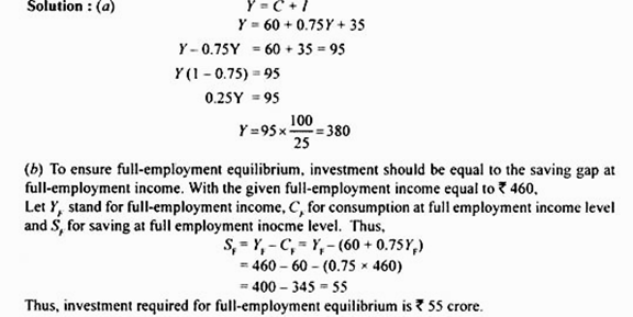
C = 60 + 0.75 Y.

(a) If investment in a year is Rs. 35 crores what will be the equilibrium level of income or output?

(b) If full-employment level of income (i. e. level of potential output) is Rs. 460 crores what invest­ment is required to be undertaken to ensure equilibrium at full-employment.

Problem 4:

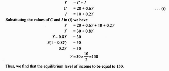
Suppose the consumption of an economy is given by C = 20 + 0.6Y

The following investment function is given: 1= 10 + 02 Y

What will be the equilibrium level of national income?

Solution:

Note that in this problem, investment varies with income. However, this will not change our method of determining equilibrium level of income.

National Income and Employment:

In our above analysis we have explained the determination of level of national income. Now, how in Keynes’s model of determination of level of employment in the economy is related to the de­termination of national income. In fact, the levels of national income and employment are determined jointly.

It will be appropriate if we now explain their determination jointly by aggregate demand and supply. It is worth nothing that, in Keynesian theory, employment is a function of income. Relation between income and labour employment is given by short-run production function showing diminish­ing returns to labour.

This short-run production function can be stated as under:

Y = f (N, K, T)

According to the above function, given the capital stock and technology, the greater the level of national output (i.e. income or Y), the greater will be the number of workers (N) employed. According to Keynesian theory, levels of national income and employment are determined by aggregate effective demand. In a closed economy with no interven­tion by the government, aggregate demand consists of consumption demand and investment demand.

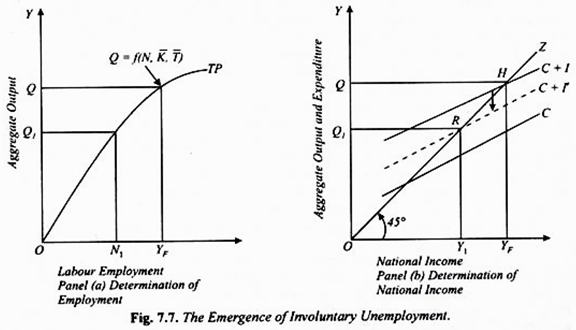
According to Keynes, consumption function is stable in the short run and it is investment demand which is highly volatile in the short run as it depends on profit expectations of business men. Equilib­rium at full employment level of income is determined when investment expenditure fills the saving gap at full employment level of national income. Consider Fig. 7.7 where in Panel (b) determination of national income is shown through intersection of aggregate demand and aggregate supply curves.

According to Keynes, equilibrium at full-employment level of income OY_F will be determined if planned investment expenditure by entrepreneurs is equal to saving gap at full-employment level of national income OY_F Total expenditure (i.e., aggregate demand) and output produced are both equal to OQ corresponding to equilibrium point H, (OQ = OY_F).

In the left-side Panel (a) where produc­tion function curve TP has been drawn , we have measured employment of labour on the X-axis and aggregate output (i.e., national income) on the K-axis. It will be seen from this left-side panel (a) that aggregate output OQ is produced by employing ON_F amount of labour. We assume that ON_F represents full employment of labour, that is, all workers who want to work at the prevailing wage rate are getting employment. With this full employment of labour, national income equal to OY_F is being generated (OY_F = OQ).

Now, Keynes argued that if somehow or the other profit expectations of entrepreneurs become dim, this would cause a fall in the expected rate of return resulting in reduction in investment expenditure. With the fall in investment expenditure, aggregate demand curve shifts downward to the dotted position C + I which intersects 45° line OZ at point R. As a result, new equilibrium level of national income OY₁is determined (OY₁ = OQ₁).

It will be seen from left side panel (a) that aggregate output (i.e., national income) OQ₁is produced by employing ON₁ amount of labour. Thus, as a result of fall in aggregate demand, N ₁N_F. number of workers are rendered unemployed. N₁ N_F workers will be involuntarily unemployed.

According to Keynes, there is no any mechanism which should ensure that this involuntary unemployment will be automatically eliminated. There is therefore need for intervention by the government.

Anti-Recessionary Policy: Shifting Aggregate Expenditure Curve Upward

Now, an important question is what measures can be adopted to overcome recession or involuntary unemployment which comes into existence as a result of deficiency of aggregate demand brought about by a fall in investment.

From our above analysis it is clear that increase in equilibrium level of national income can be brought about by increases in any components of aggregate demand, namely, consumption demand (C), private investment demand (I), Government expenditure (G), and net exports (NX).

In order to increase national income through upward shift in the consumption function, the Government can reduce personal income taxes. In 1964, the reduction in income tax by John Kennedy Government in USA was quite successful in boosting consumption demand and thereby raising aggregate output. As a result, more income and employment were generated.

The rate of unemployment sharply declined and the American economy was lifted out of depression. Recently, in 2002 and again in early 2008, the President George W. Bush made a significant cut of 3.5 billion dollars in income tax to revive the American economy. He refunded a good amount of income tax collected from the people in these years.

The cut in direct taxes increases the disposable income of the people which tends to raise their consumption demand. However, there is a limitation of cut in direct taxes for raising aggregate demand because a part of the increase in disposable income can be saved rather than being spent on goods and services.

This happened in the United States in the year 2008. To boost aggregate demand, indirect tax can also be also be reduced. In India also, in December 2008, to correct the sagging demand for industrial products the Government under the fiscal stimulus package made 4 per cent across the board cut in central excise duty. This too has a limitation because benefit of this cut in excise duty may not be fully passed on to the consumers by reducing prices.

Secondly, the equilibrium level of national income (GNP) and employment can be increased by raising the rate of private investment (I). Through monetary policy measures businessmen can be induced to invest more by lowering the rate of interest and increasing the availability of credit. We know that the lower the rate of interest, the higher will be the level of private investment. Alternatively, the Government may encourage private investment by reducing tax on profits so that post-tax rate of profit will be higher than before. The higher level of investment will shift the aggregate expenditure curve (C +1+ G) upward and determine a higher level of national income and employment.

Thirdly, the recession can be overcome and national income (GNP) and employment can more efficiently be increased by increasing Government expenditure (G). It was the increase in Govern­ment expenditure on Public Works Programme which was the main recommendation of Keynes to raise the level of national output and income to restore equilibrium at full-employment level. Recently in 1993-94, President Clinton stepped up public expenditure on public works in the USA to overcome recession in the American economy and reduce unemployment.

Again in 2009 president Obama planned to give a fiscal stimulus of over $ 800 billion the major part of which was the increase in Government expenditure to raise aggregate demand to overcome recession in the American Economy. In India also fiscal stimulus packages were announced in 2008-09 under which government expenditure, especially on infrastructure projects, was increased to revive slowing Indian economy.

Lastly, the expansion in positive net exports (NX) will also cause an increase in equilibrium level of national income and employment. Exports can be promoted through tax concession on profits earned through exports as well as making credit available on lower interest rate for purpose of exporting goods.

Another common measure adopted to promote exports is the depreciation of national currency. Depreciation makes the exports cheaper and imports costlier which raise net exports (NX). However, when there is global recession depreciation of its currency by each country will offset the effect of others. It follows from above that a mix of fiscal and monetary policy measures are adopted to increase in aggregate expenditure and demand and thereby to lift the economy out of recession.

Determination of National Income: Saving-Investment Approach:

We have seen how equilibrium level of national income is determined by the interaction of aggregate demand and aggregate supply. The equilibrium level of national income is established at the point where aggregate demand equals aggregate supply. But there is an alternative method for the explanation of the determination of national income. This alternative method explains the determina­tion of national income directly by intended saving and investment.

Look at the Fig. 7.5 again. In this figure, at the equilibrium level of national income OY_1,saving and investment are equal to GE. Given the aggregate demand curve C + I, the amount of saving at income greater than OY₁ exceeds investment and for income less than OY₁ investment exceeds saving.

It is obvious that intended saving and investment are equal only at the equilibrium level of national income and when intended saving and investment are not equal, national income will not be in equilibrium. Let us see why it is so and how national income is determined by intended saving and investment.

When at a certain level of national income, intended investment by the entrepreneurs is more than intended saving by the people, this would mean that aggregate expenditure is greater than aggregate supply of output. This will lead to the decline in inventories below the desired level. This would induce the firms to increase production, raising the level of income and employment.

The result will be that national output will be increased on account of which national income will go up. Further, when at any level of income, investment is less than saving. It means that aggregate demand is less than aggregate supply. As a result, the entrepreneurs will not be able to sell their entire output at given prices. The result will be that output will be reduced which will result in the reduction of national income.

Thus, when, at any level of national income, investment demand of the entrepre­neurs is less than the intended savings of the people, the national income will decrease. It will come down to the level at which investment spending is just equal to the planned savings by the community.

But, when at any level of national income, intended investment demand on the part of the entrepreneurs is equal to intended savings of the people, it means that aggregate demand is equal to the total output or aggregate supply and therefore the national income will be equilibrium. Hence, equilibrium level of national income will be determined at the level at which the amount of intended investment by the entrepreneurs is equal to the amount of intended savings by the people.

We can explain the determination of national income through saving and investment in another way. Saving represents withdrawal of some money from the income stream. On the other hand, investment represents injection of money into the income stream. Now, if intended investment is greater than intended saving, it means that more money has been put into the income stream than has been taken out of it. As a result, income stream, i.e., flow of national income would expand.

On the contrary, if investment is less than intended saving, it means that less amount of money has been put into the income stream than has been taken out of it. The result would be that national income would decrease. But when investment is just equal to saving, it would mean that as much money has been put into the income stream as has been taken out of it.

The result will be that the national income will neither increase nor decrease, i.e., it will be in equilibrium. It is thus clear that the equilibrium level of national income will be determined at the level at which the intended investment is equal to intended saving.

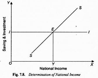
The determination of national income by investment and saving is illus­trated in Fig. 7.8. In this figure, national income is shown along the X-axis. SS is the saving curve which shows intended saving at different levels of income, II curve shows investment demand i.e., intended investment. The II investment curve has been drawn parallel to the X-axis. This is done on the assumption that in any year the entrepreneurs intend to invest a certain amount of money. This implies that we assume that investment is independent of change in income, that is, investment does not change with income.

The saving curve SS and the investment curve II intersect each other at E. That is, the intended investment and intended saving are equal at the OF level of income. Hence, OY is the equilibrium level of income. It will be seen from the Fig. 7.8 that at the level of income less than OY, the amount of intended investment is more than intended savings. As a result, income will increase.

On the contrary, at the level of income a greater than OY, the amount of intended investment is less than the intended savings with the result that income will decrease. The decrease in income will continue until it becomes equal to OY. At the level of OY income, intended investment and intended saving are equal, so that there is neither the tendency for income to increase, nor to decrease. Hence, national income OY is determined. It is thus clear that national income is determined by the investment and saving.

Synthesis between the Two Approaches:

The determination of national income has been explained above by two methods.

The equilib­rium level of national income is determined where two conditions are fulfilled:

(i) Aggregate Expenditure or Demand = Aggregate Supply of output, and

(ii) Intended Investment = Intended Savings.

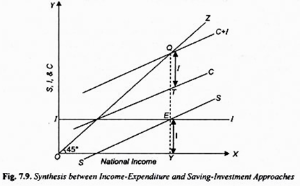
The equality between aggregate expenditure and aggregate supply of output and equality between intended investment and intended saving in reality mean the same thing. This is illustrated in Fig. 7.9. It will be seen in this figure that aggregate demand curve C + I intersects aggregate supply curve OZ at point Q and thereby determines national income equal to OY. In the lower part of this diagram we have draw intended savings curve SS and intended investment curve II.

It is worthwhile to note that saving curve SS has been derived from the consumption function curve C and measures the gap between income and consumption at various levels of income. Further, investment curve II drawn in the lower part of the figure represents the difference between consumption function curve C and aggregate demand curve C + I.

This difference is the amount of intended investment assumed in this figure. We thus see that both saving and investment curves drawn in the lower part are embedded in the upper part showing aggregate demand and aggre­gate supply. It is because of this that intended saving and intended investment curves also determine the same level of national income OY which is determined through the equality of aggregate demand (C + I) and aggregate supply.

Saving-Investment Approach: Algebraic Analysis:

That the level of national income is determined by the equality of planned saving and planned investment can be derived from the equilibrium condition explained above that level of income is equal to effective demand.

That is,

Y = AD* … (i)

Where AD* represents effective aggregate demand or expenditure

Now in our simple economy, effective aggregate demand (AD*) is equal to the sum of consumption expenditure and investment expenditure. Thus

AD* = C + I

or y = C + I …(ii)

Now C = Y – S

Substituting Y— S for C in equation (ii) we have

Y = Y – S + I

Y – Y + S = I

o r S = I … (iii)

Thus, we reach at the alternative condition of equilibrium of national income, namely, planned (intended) saving be equal to planned (intended) investment. We can further extend saving – investment approach to show the determination of national income as a multiple of autonomous factors. Since investment is treated as autonomous of national income, its amount is taken to be a fixed amount determined exogenously. Therefore we have

I = I

Saving function as derived from the consumption function (C = a + by) can be written as:

S = -a + (1 – b) Y

In equilibrium

I = –a + (1 – b)Y

(1 – b)Y = I + a

Y = 1/1 – b (I + α)

where 1/1 – b is the value of multiplier and b = marginal propensity to consume and therefore 1 – b = marginal propensity to save. The equation (iv) describes the same condition which we at derived earlier. Note that a in equation (iv) is autonomous consumption which is intercept term in the consumption function.

Numerical Problem on Saving-Investment Approach:

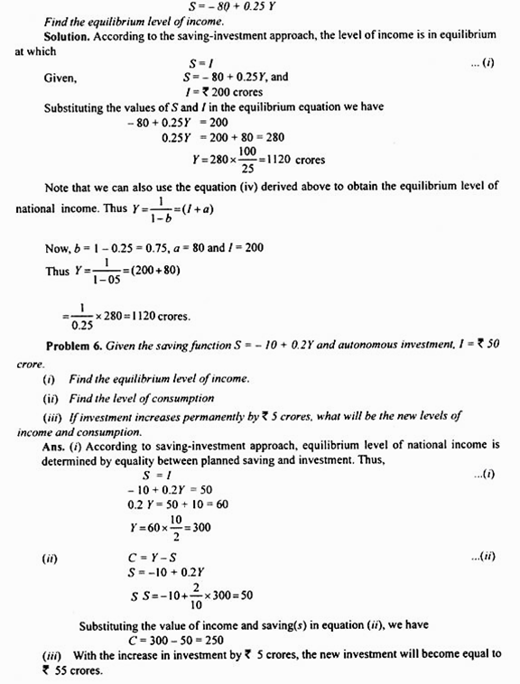
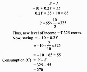
Suppose the level of autonomous investment in an economy is 200 crores.

The following saving function is given: