Let us make in-depth study of the three sector and four sector models in determination of national income of a country.
Determination of National Income: Three Sector Model:
Government Expenditure and National Income:
The equilibrium level of national income is determined by the consumption function and autonomous investment demand.
However, in all economies today including the free-market capitalist economies such as those of U.S.A., Britain, Japan, the Government expenditure on goods and services plays an important role in the determination of national income and therefore it should also be included in the analysis of income determination.
It is important to note here that the magnitude of Government expenditure on such things as highways, public parks, education, health services is governed by the consideration of promoting social welfare, employment and growth in the economy and does not depend on the level of income of the economy. Therefore, in the simple Keynesian model of income determination, the Government expenditure is treated as autonomous expenditure.
ADVERTISEMENTS:
We further assume for the moment that Government spends on goods and services but imposes no taxes. We denote Government expenditure by G.
Thus in the three sector economy when we take into account the income generating effects of Government expenditure, we get the following equation for the equilibrium level of national income.
Y = C + I + G
where Y is national income or output and C + I + G represents the level of aggregate demand including Government expenditure, G.
ADVERTISEMENTS:
Since consumption function C = a + bY where b stands for marginal propensity to consume and a for autonomous consumption expenditure, we can rewrite the equilibrium level of national income as under:
Y = a + bY + I + G
Y – bY = a + I + G
Y(1 – b) = a + I + G
ADVERTISEMENTS:
K (a + I + G)
Thus it is clear that the equilibrium level of income (when impact of Government expenditure is also considered) is equal to the sum of three types of fixed autonomous expenditure, namely, autonomous consumption, autonomous investment and Government expenditure (a + I + G) multiplied by mous consumption, autonomous investment and Government expenditure (a + I + G) multiplied by the value of the multiplier [1/(1 – b)].
Graphic Illustration:
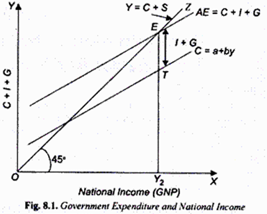
The impact of Government expenditure on goods and services on the equilibrium level of national income is illustrated in Fig. 8.1. C is the consumption function curve to which we have added the autonomous investment equal to I. On top of the consumption demand C and investment demand I, we have added the Government expenditure on goods and services (G) to get the aggregate expenditure (or aggregate demand) curve C + I + G.
With this, the equilibrium national income OK, is determined at the level at which the aggregate expenditure curve (C + I + G) interests the 45° line, that is, aggregate expenditure (C + I + G) equals aggregate supply of output. The reason for the determination of equilibrium level of income at OK, when Government expenditure is included in the aggregate expenditure curve is the same as stated earlier.
It will be observed from Fig. 8.1 that at a level of national income less than OK, aggregate expenditure C + I + G exceeds aggregate supply. This implies unintended decline in the inventories of goods with the firms which will induce them to expand the level of aggregate output to the level OY2.
On the contrary, at the level of national income greater than OY2 the aggregate expenditure is less than aggregate supply of output. This deficiency of demand for goods will cause unintended accumulation of inventories. The firms would respond to this by cutting back production of goods which will lead to the reduction of national income to OY2
It is important to note that in the presence of Government expenditure, national income is determined at the level at which the saving gap is equal to the sum of private investment and Government expenditure (I+ G). It will be seen from Fig. 8.1 that at OK, equilibrium level of national income (GNP), the saving gap is TE which is equal investment and government expenditure. It may be further noted that just as investment expenditure has a multiplier effect on increase in income Government expenditure too has a multiplier effect.
Government Expenditure, Budget Deficit and Capital Market:
ADVERTISEMENTS:
We know how the government expenditure affects the product market by bringing about increase in aggregate demand. Now, an important question is how the Government expenditure is financed. Imposition of taxes is an important way of financing Government expenditure.
But taxes reduce aggregate demand in the product market by lowering disposable income of the community and thereby causing a decline in its consumption expenditure. Therefore, if Government expenditure equals tax revenue collected (G = T), then Government has a balanced budget and much of the expansionary effect of government expenditure is offset by taxes levied.
If Government increases its expenditure without raising taxes, (i.e. G > T), then it has a budget deficit which has a large expansionary effect on the product market and, as seen above, leads to increase in national income (GDP). This deficit budget is often financed by borrowing from the public. But borrowing by the Government to finance its deficit affects the capital market.
This is because borrowing by the Government will compete with private investors for the savings of the public. As a result of borrowing by the Government from the market, less saving is available for private investment.
ADVERTISEMENTS:
When the Government runs a deficit, private saving has two uses:
(1) To finance private investment and
(2) To finance Government budget deficit which is met by borrowing from the public?
Equilibrium in the capital market occurs when private saving is equal to private investment plus budget deficit, G – T, (i.e. Government borrowing).
ADVERTISEMENTS:
Thus, in equilibrium in the capital market
Sp = I + (G – T)
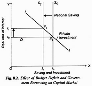
where Sp stands for private saving, I for private investment, and (G – T) stands for budget deficit (i. e. Government borrowing). How budget deficit or Government borrowing reduces or crowds out private investment is illustrated through Figure 8.2 where to begin with vertical saving curve S0 intersects the downward-sloping investment curve II at point E0 and determines real interest rate r0at which private investment equal to I0 takes place.
Now, as a result of Government borrowing to finance its budget deficit (G – T) saving available for private investment falls and the national saving curve shifts to the left to the new position Sv Note that when Government borrows to finance budget deficit, Government is said to dis-save and therefore in this case Government or public saving is negative (G – T = – Sg). Note further that national saving = private saving and Government saving (S = Sp + Sg).
That is why when Government borrows (i.e. dis-save), national saving curve shifts to the left to S1The capital market is now in equilibrium at point E1 and rate of interest rises to r1 At this higher interest rate r1, private investment falls to I1. Thus, borrowing by the Government to finance its budget deficit has led to crowding out of private investment. A part of private saving is used to finance private investment and a part to finance budget deficit of the Government.
It is worth noting that when Government expenditure is fully matched by increase in taxes (i.e. G = T) we have a balanced budget but it will still have a expansionary effect on national income, though, as shall be explained below, the multiplier effect of a balanced budget is equal to one. However, since in case of balanced budget increase in Government expenditure is matched by increase in taxes which reduces disposable income Yd = Y – T. And reduction in disposable income (Yd) leads to decrease in both consumption and saving (Yd = C + S). This decrease in private saving will cause rate of interest to rise and thereby crowds out private investment.
ADVERTISEMENTS:
Further, when the Government has a budget surplus (i.e. T > G), it has a positive saving which will lead to the increase in national saving and make more funds available for private sector to borrow. This will cause real rate of interest to fall. As a result, higher private investment will occur in case of surplus budget.
It is worth noting that in our above analysis Government expenditure has been treated as consumption expenditure on goods and services purchased to satisfy collective wants. However, this is strictly true in case of a purely free- market economy such as that of the US where the Government is not a major investor.
But in case of India’s mixed economy the Government is an important investor and a good part of its borrowing is used for investment purposes, especially for investment in infrastructure projects such as power, transport, highways, roads, ports etc. Such Government borrowing for investment purposes cannot be considered as consumption expenditure or dissaving.
Therefore, it has a large expansionary effect on national income with a usual multiplier effect. Viewed as such Government borrowing for investment, especially tor infrastructure projects in developing countries, may crowd in private investment rather than crowding it out. This is so because lack of adequate infrastructure hinders private investment.
Determination of National Income with Government Expenditure and a Lump Sum Tax:
Now in a three sector model we analyse the impact of Government expenditure when to finance this expenditure the government levies a lump sum tax. Note that a lump sum tax does not vary with income. In this case if government expenditure equals revenue from lump-sum tax, its budget will be in balance.
ADVERTISEMENTS:
On the other hand, if government expenditure exceeds tax revenue, there will be a deficit budget. Further, if tax revenue is more than its expenditure, government will have a surplus budget. We are here concerned with the impact of government expenditure and taxation on the determination of national income.
Let us assume the government follows a balanced budget policy in which case government expenditure equals tax revenue from lump sum tax. Let us assume that there are no transfer payments made by the government.
Three sector model with the above specifications can be developed as follows:
Y = AD = C + I + G
or Y = C + I + G …(i)
Now, consumption function can be stated as:
ADVERTISEMENTS:
C = a + bYd
Where a is constant autonomous consumption expenditure, Yd is disposable income.
In this three sector model with lump sum tax and no transfer payments, consumption function can be written as:
C = a + b (Y — T)
where T = lump sum tax
or C = a + bY – bT
ADVERTISEMENTS:
Substituting the value of C in income equation (i) we have:
Y = a + bY – bT + l + G
Y – bY = a – bT – l + G
Y(1 – b) = a – bT + I + G
Y = -(1/ a – b (a – bT + I + G)
The equation (ii) furnishes us the equilibrium level of national income in the three sector economy when there is both government expenditure and lump sum tax. Therefore, for an economy if the data regarding consumption function, investment, Government expenditure and lump sump tax are given we can compute the equilibrium level of national income. A numerical example will clarify the determination of equilibrium level of income in this case.
Problem 1:
The following data characterizes the macroeconomic conditions of a hypothetical economy:
C = 50 + 0.8 yd
I = 100
G = T = 75
where C, I, and Yd are consumption, investment and disposable income respectively.
Calculate equilibrium income of the economy. What is the value of multiplier?
Solution:
Note that since G = T, budget of the Government is balanced.
Y = C + I + G
C = a + bYd = a + b(Y – T)
Substituting the values of C, I and G we have:
Y = 50 + 0.8 (Y – 75) + 100 + 75
= 50 + 0.87 – 60 + 100 + 75
Y = 165 + 0.8Y
Y – 0.8Y = 165
Y (1 – 0.8) = 165
0.2 Y = 165
Y = 165 x 10/2 = 825
Thus, equilibrium level of income is 825.
Since in the present problem G = T, budget is a balanced one
Value of balanced budget multiplier = 1/1 – b + -b/1 – b
where b represents marginal propensity to consume. In the given consumption function,
b = 0.8
Value of balanced budget multiplier 1/1 – 0.8 + -0.8/1-0.8 = 1/0.2 – 0.8/ 0.2
= 5 – 4 = 1
Determination of National Income in the Three Sector Economy with Lump Sum Tax And Transfer Payments:
We have explained above the determination of national income in the three sector economy when government expenditure is financed by imposition of lump sum tax. We now extend our model to include transfer payments and see how they affect determination of national income.
Transfer payments are payments to the people by the government for which it receives no service or goods in return from them. Transfer payments are made by the government to promote social welfare. Unemployment allowance, poverty relief grants, social security contributions, old age pension are some important examples of transfer payments. Transfer payments are antithesis of tax. Whereas tax reduces disposable income of the people, transfer payments increase their disposable income.
Transfer payments may be autonomous of tax or they may be financed by imposition of a lump sum tax. If, like the government expenditure on goods and services, transfer payments are financed through tax, then transfer payments become a part of government expenditure (G) and imposition of additional tax to finance transfer payments become a part of total lump sum tax (T) which reduces disposable income.
Therefore, in this case when transfer payments are financed through additional taxes, the analysis of income determination is similar to the model of income determination with government expenditure and lump sum tax explained above. However, the inclusion of transfer payments which are of autonomous type makes the analysis of income determination somewhat different. We describe it below.
Since transfer payments increase the disposable income of the people, they will increase their consumption expenditure depending on their propensity to consume. Thus
C = a + bYd
Yd = Y – T + TR
where T is lump sum tax and TR is transfer payments
C = a + b (Y – T + TR)
Y = C + 1 + G
= a + b(Y – T + TR) + I + G
Y = a + bY – bT + bTR + I + G
Y – bY = a – bT + bTR + I + G
Y (1 – b) = a – bT + bTR + I + G
Y = 1/1 – b (a – bT + bTR + I + G)
Government Expenditure Multiplier and Transfer Payments Multiplier:
It is important to note that the multiplier of government expenditure on goods and services is different from transfer payments multiplier. This is because whereas Government expenditure on goods and services raises aggregate demand directly by its full amount, the transfer payments raises consumption demand by bTR, that is, less than the full amount depending on the marginal propensity to consume. Let us illustrate it by using income equation (ii).Suppose government expenditure increases by AG. Then, increased income is
Y + ∆Y = 1/1-b (a – bT + bTR + I + G + ∆G)
Subtracting equation (ii) from equation (iii) we have:
∆Y = 1 – 1/b (∆G)
∆Y/∆G = 1 /1 – b
Thus, Government expenditure multiplier, ∆Y/∆G = 1/1-b
where b is marginal propensity to consume.
If instead of increasing government expenditure on goods and services, government increases transfer payments by ATR we will get the following income equation
Y + ∆Y = 1 – 1/b (a -bT + bTR + b∆TR + I + G)
Subtracting equation (ii) from equation (iv) we have:
∆Y= 1/1 – b b∆TR
Or ∆Y/∆TR = b/1 – b
Thus, transfer payments multiplier, ∆Y/∆TR = b/1 – b
Taking the difference between the Government expenditure multiplier and transfer payments multiplier we have:
1/1 – b – b/1 – b = 1 – b/1 – b = 1
Problem 2:
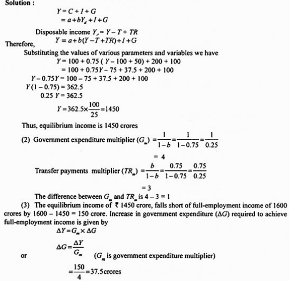
Suppose the structural model of an economy is given below:
C = 100 + 0.75 Yd
I =200
G = T = 100
TR = 50
where G is government expenditure on goods and services, T is lump sum tax and TR are transfer payments:
(1) Find the equilibrium level of income
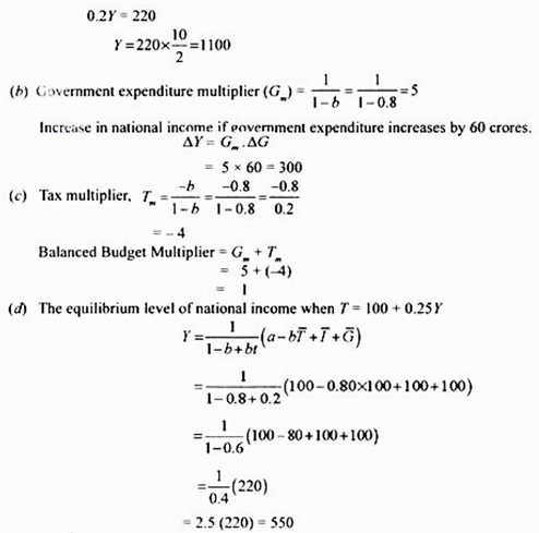
(2) Calculate Government expenditure multiplier and transfer payments multiplier. What is the difference between the two?
(3) If full-employment level of income is 1600 crores, how much government expenditure be increased to attain full employment?
Three Sector Model Further Extended:
In our above analysis of determination of equilibrium national income in a three sector economy we have assumed autonomous constant investment, apart from consumption function of households and Government expenditure on goods and services and transfer payments.
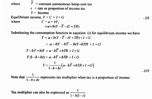
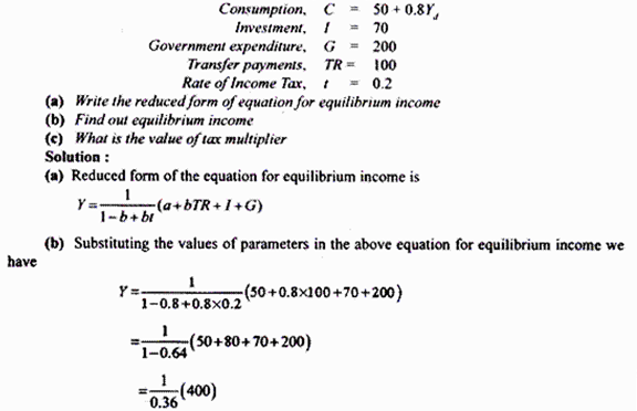
In the further extension of the model we also include proportional income tax, that is, a tax levied as a proportion of income. Proportional income tax is therefore expressed as tY where t is the rate or proportion of income which is payable as a tax. In a real economy proportional income tax may be imposed along with any lump sum tax.
Thus, the total tax (T) can be expressed as:
T – T + tY
Problem 3:
For a closed economy, the following data is given:
The Lump-sum Tax Multiplier:
We have explained the multiplier effect of change in Government expenditure on goods and services and of change in transfer payments (TR) on the equilibrium level of income. We will now explain the multiplier effect of change in tax. Reduction in taxes has often been used by the policy makers to increase aggregate demand of the economy and thereby to lift the economy out of recession.
For example, in 1964 John F Kennedy, the president of the United States made a substantial cut in personal and corporate taxes to stimulate expenditure on consumption and investment to bring about expansion in income and employment in the economy. This policy of cut in taxes to revive the American economy had a grand success. There was a large growth in Gross Domestic Product (GDP) of the United States in 1964 and 1965. There was a substantial fall in unemployment as a result of the policy of cut in taxes.
Recently when George Bush was elected president in 2001 the American economy found itself in the grip of recession. He also made a drastic cut in income tax to stimulate aggregate demand so as to overcome recession. Again this policy of tax cut was greatly successful and the American economy recovered in 2003-04.
The change in lump sum income tax and proportional income tax affect equilibrium income differently, but both have a multiplier effect on equilibrium income. We have already explained the effect of lump-sum income tax and proportional income tax on the equilibrium level of income.
We are now concerned with analyzing the effect of change in lump sum tax and proportional income tax. For the sake of simplicity and convenience we explain the multiplier effect of lump sum income tax. Note that while a cut in tax will have a positive effect on equilibrium income, increase in tax will reduce equilibrium income. Suppose the government increases lump-sum income tax by AT we are interested to know its multiplier effect on income.
As found above, in the three sector economy with Government expenditure and lump-sum tax:
Y = 1/1 – b (a – bT + I + G)
where 7 is lump sum income tax. Now, a decrease in lump-sum income tax by ∆T will cause a change in income (that is, ∆Y). Increase in tax will reduce the disposable income and therefore the consumption demand. As a result of increase in tax, consumption demand will decrease by the change in tax times the marginal propensity consume, that is, ∆Y= bAT. Let us incorporate change in the tax (AT) in the three sector equation (1) for equilibrium income and see how much change in income (AY) it brings about. Thus
Y + ∆Y = 1/1 – b [a – b (T + ∆T) + I + G]
Y + ∆Y = ∆Y (a – bT – b∆T + I + G) … (2)
Now subtracting equation (1) from equation (2) we have:
∆Y = 1/1 – b (-b ∆T)
Dividing both sides by ∆T we have:
∆Y/∆T = -b/1-b …(3)
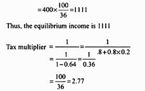
∆Y/∆T is the expression for tax multiplier. It will be seen that increase in tax by ∆T will reduce equilibrium income by a multiple. For example, if marginal propensity to consume is 0.75, then the tax multiplier is
∆Y/ ∆T= -b/1-b = -0.75 /1-0.75= -0.75/0.25 =-3
This means that increase in tax by Rs .1 will cause a decline in equilibrium income by 3. Note that we can similarly prove that a cut in tax will raise the equilibrium income through the tax multiplier. Therefore, in case of reduction in lump sum income tax, the tax multiplier is ∆Y/∆T= b /1-b
With 0.75 as marginal propensity to consume, tax multiplier of cut in tax is,
∆Y /∆T 0.75/1- 0.75= 30.75 / 0.25 = 3
Balanced Budget Multiplier:
We now analyse the impact of balanced budget of the government. In case of a balanced budget, the government’s expenditure is equal to its tax revenue, that is, G = T and therefore when the government increases its expenditure by ∆G, then it also raises taxes to get more tax revenue (∆T) so that ∆T = ∆G. The effect of a balanced budget on the equilibrium income is described by the balanced budget multiplier which is also called balanced budget theorem.
According to this, the balanced budget multiplier is always equal to one. We prove it below by assuming a lump sum tax. In order to analyse the effect of a balanced budget multiplier, we reproduce below the equation for equilibrium income for a three sector economy.
Y= 1/1 – b (a – bT + I + G)
where T is constant lump sum tax levied by the government.
Let us incorporate increase in government expenditure (∆G) fully financed by additional lump sum tax (∆T), that is, ∆G = ∆T.
By doing so we get:
Thus, balanced budget multiplier is equal to one. This implies that when ∆G = ∆T and budget is therefore balanced, national income increases by the same amount as the increase in government expenditure.
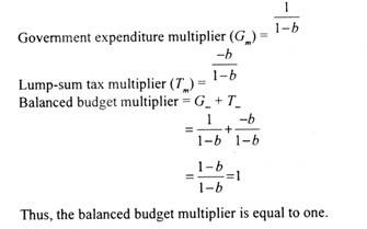
Alternative Proof:
That the balanced budget multiplier is equal to one can be proved in an alternative way. Balance budget multiplier is the sum of government expenditure multiplier and lump sum tax multiplier.
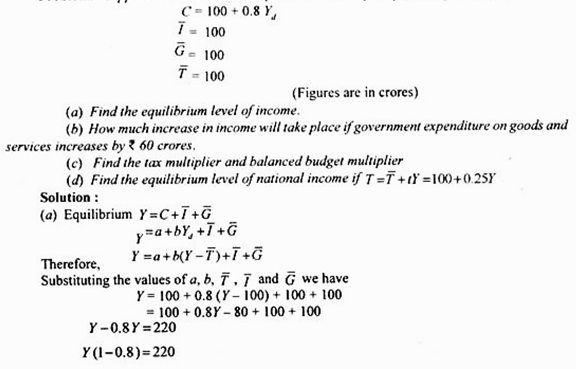
Problem 4:
Suppose we have an economy characterised by the following functions:
Determination of National Income in an Open Economy: Four Sector Model:
In modern times economies of different countries are integrated with each other though some are more integrated than others. An open economy is one which has not only trade relations with other countries but has financial capital flows between it and other economies of the world.
It is because of such openness and integration of the economies of the world that recent financial crisis that occurred in the United States in 2007 has significantly affected other economies (including that of India) causing global meltdown through its affect on trade and capital flows. Under capital flows, funds flow from one country to another. Foreign trade of goods and services affect product market and influences the determination of national income of a country as net exports (i.e. exports-imports) is a part of aggregate demand for output produced by an economy.
On the other hand, capital flows in an open economy provide funds for financing domestic investment or for financing government budget deficits or for financing current account deficit. If the demand for funds in an economy exceeds domestic national saving, the private sector and Government of an open economy can get them from abroad either through borrowing or direct or portfolio investment by foreign investors. We start with the analysis of impact of inclusion of foreign trade on the determination of national income of a country.
Foreign Trade and National Income in an Open Economy:
In the four sector model of determination of national income, we add the foreign trade sector to the three sectors, namely, households, firms, and Government. Foreign trade, that is, volume of exports and imports of a country also affects the level of national income of a country. We now extend the Keynesian model of determination of national income by including the effect of exports and imports of a country on the generation of income.
For example, the exports of India represent the foreign demand and generate income for the Indian people. On the other hand, imports represent the demand for foreign goods by the Indians and generate incomes for the people of other countries. Therefore, imports tend to reduce the domestic aggregate expenditure. It therefore follows that national income will depend on the net exports, that is, exports minus imports (X – M) where X stands for exports and M for imports.
The exports and imports of a country depend to a great extent on the level of economic activity (that is, the level of output and income of the country). Thus, when the growth of industrial output in India is rapid, it will generate greater demand for imported materials. On the other hand, the higher industrial growth would also cause our exports to rise provided there is demand for our goods abroad.
However, in the Keynesian model of income determination, exports and imports are considered as autonomous, that is, independent of income, being determined outside the model. Further, as mentioned above, the increase or decrease in aggregate expenditure or demand due to exports and imports depends on the net exports, that is, X – M which we may write as NX. If the net exports are positive, there will be addition to the aggregate demand or expenditure of a country. On the other hand, if the net exports are negative, there will be decrease in aggregate expenditure.
When we include net exports (X) in our analysis we get the following equation for the equilibrium level of income.
Y = C + I + G + (X – M) where
C = a + b(Y – T)
Y = a + bY – bT + I + G + NX
or Y(1 – b) = a – bT + I + G + NX
Y = 1/1 – b (a – bT + I + G + NX)
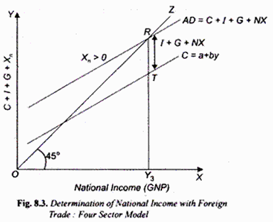
Thus, the equilibrium level of income is the sum of all fixed autonomous expenditures (i.e., a – bT + I + G + X) times the value of multiplier [1/1 – b]. It is worth noting that in the four sector model, national income is determined at the level at which saving gap between consumption and income is equal to the sum of investment, Government expenditure and net exports, (that is, I + G + Zn).
Graphic Illustration:
In Fig. 8.3, we have depicted the determination of national income when there are positive net exports (that is, when exports exceed imports, X – M> 0. To obtain the aggregate demand curve incorporating the positive net exports (NX) we add the I + G + NX to the consumption function curve C to get the higher aggregate demand curve C + I + G + NX which intersects the 45° line at point R and determines a level of income OY3 If the net exports AX were negative, that is, imports exceed exports, X-M < 0, the aggregate demand curve incorporating net exports would lie at a lower level than C + 1 + G curve and determine a lower level of income.
Trade Balance (Net Exports) and International Capital Flows:
In an open economy as in the closed economy product markets and capital markets are closely related.
To know this relationship let us consider the equilibrium level of national income in an open economy which is:
Y = C + I + G + (X – M) … (i)
where X- M are net exports (NX)
Therefore, rearranging the above equation and writing NX for X— M we have:
Y – C – G = 1 + NX … (1)
Now Y-C-G represents national saving’ which we represent by S.
Writing S for national saving (Y – C – G) in equation (2) we have:
S = I + NX … (2)
or S – I = NX …(3)
From equation (3) it is evident that difference between domestic saving and domestic investment (S – f) equals net exports (NX). Since difference between domestic saving and investment (S – I) represents capital flows, equation (3) reveals that capital flows between an economy and the foreign ones are related to net exports (NX) which are also called trade balance.
If for a country domestic saving exceeds domestic investment (S > I), then the country would have positive net capital outflows which means residents of the country would be lending or investing abroad more than the foreigners would be lending or investing in the country concerned.
The equation (3) above shows that these positive net capital outflows imply that they will be equal to positive net exports (NX), that is, the country will be exporting more than it will be importing. Foreigners will need financial loans to buy that country’s more goods and services than they are exporting to it.
This has been the relationship with Japan and the US. Japan has a trade surplus (i.e. positive net exports) with the US and to enable the US to buy more Japanese goods than Japan is importing from it, it has been lending to the US which has been running a trade deficit, that is, there has been net capital outflows from Japan to the US.
Now, when domestic saving of a country is less than the domestic investment (S < I or S – I is negative), the equation (3) above reveals that the net exports (NX) will be negative (i.e., the country will have a trade deficit) and, therefore, there will be net capital inflow. The net capital inflow implies that the country will be borrowing from abroad or receiving foreign investment.
The country having negative net exports or deficit trade balance requires foreign capital funds either through borrowing from foreigners or foreign direct investment so as to enable it to import more goods and services than it is exporting to them.
For example, in India we have a deficit in the current account of balance of payments (which has the same meaning as the concept of trade balance involving both goods and services) for several years now so that foreign saving or capital inflow have contributed to the increase in investment in India though the share of capital inflows (foreign savings) as a per cent of its GDP in India is relatively small.
Foreign Trade Multiplier:
So far in our analysis of four sector model of income determination we have assumed that both exports and imports are constant autonomous items, that is, independent of income. In the model of income determination while exports are regarded as constant autonomous factor determined exogenously (that is, X = X ), imports are treated as function of two variables, namely, (1) autonomous imports (i. e. independent of income), and (2) level of income.
Thus, import function used in the model can be written as:
M – M + mY
where M represents autonomous imports, m Y represents imports dependent on level of income (Y) and m is marginal propensity to import. Given the marginal propensity to import (m), as income increases, mY will increase.
By incorporating the above import function we can derive the complete four sector model of income determination as follows:
Y = C + I + G + (X – M) …(i)
where C = a + b(Y – T)
M = M + mY
and
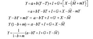
Substituting the consumption function and import function in the income equation … (i) we have:
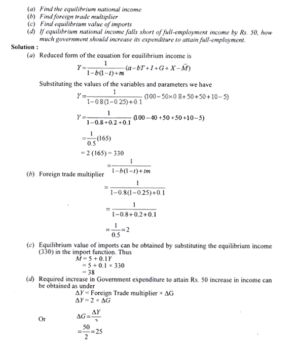
where the term 1/ 1-b+ m is known as foreign trade multiplier whose value is determined by marginal propensity to consume (b) and marginal propensity to import (m). Note that change in any autonomous factor of the model such as X, G, I, a, M will cause a change in national income by the value of multiplier 1/ 1 – b + m times the change in the amount of the factor. Thus, if exports increase by ∆X the national income will increase by ∆Y= 1/ 1- b+ m ∆X
Incorporating Proportional Income Tax in the Four Sector Model:
If in the above four sector model of income determination proportional income tax is incorporated, then only the term of foreign trade multiplier will change, the other terms of the model remaining the same. Thus, if income tax is of form T = T + tY where T is constant lump sum, t is the proportion of income that is taken as tax.
With incorporation of proportional income tax, the value of foreign trade multiplier becomes:
= 1/1-b (1-t) +m
= 1/1-b + bt+ m
or
where t is the proportional income tax rate.
With this proportional income tax, the above equilibrium income equation can be written as:
Y =1/ 1-b (1-t)+ m (a-bT + I+O + X-M)
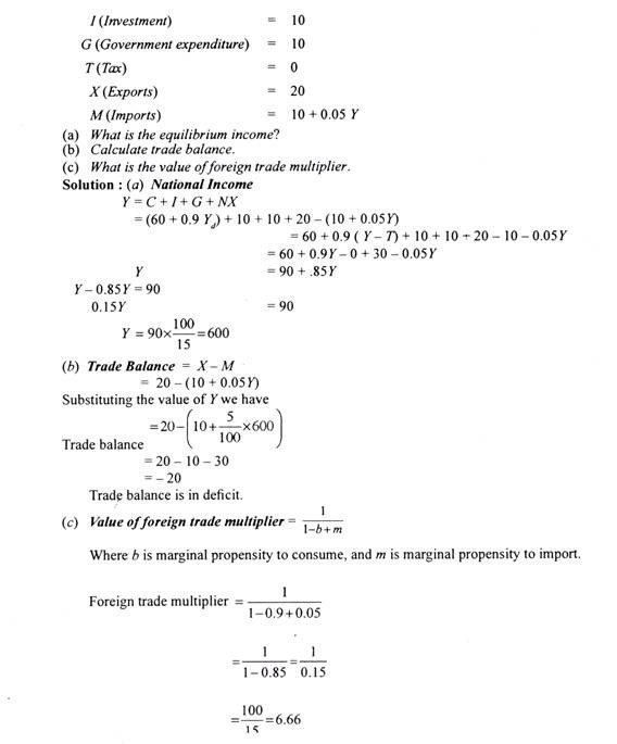
Problem 5:
An economy is characterised by the following equations:
C (Consumption) = 60 + 0.9 Yd
Problem 6:
Behavioural and structural equations of an economy are given below:
Economic Policy Implications of Keynesian Analysis of National Income:
Keynesian analysis of determination of national income is highly relevant and of great practical use in the formulation of economic policy to overcome recession or depression in the economy and also to solve the problem of inflation in the economy. A free market economy often faces the problem of recession or slowdown in the economic activity at sometimes and to contend with the problem of severe inflation at other times.
From our above analysis it is clear that changes in equilibrium level of national income can be brought about by changes in any component of aggregate demand, namely, consumption demand (C), private investment demand (I), Government expenditure (G), and net exports (Xn). In order to increase national income through upward shift in the consumption function, the Government can reduce personal income taxes.
In 1964, the reduction in income tax by John Kennedy Government in USA was quite successful in boosting consumption demand and thereby raising aggregate output. As a result, more income and employment were generated. The rate of unemployment sharply declined and the American economy was lifted out of depression. Recently in 2002, the President George W. Bush made a cut of 3.5 billion dollars in income tax to revive the American economy.
This also proved quite successful. Again in 2007-08 the American President made a drastic cut in income tax to increase demand for getting the US economy out of recession which was caused by financial crisis brought about by defaults in payment by the people of sub-prime housing loans. In India too government cut excise duties and service tax under fiscal stimulus package to prevent sharp slowdown of the Indian economy.
Secondly, the equilibrium level of national income (GNP) and employment can be increased by raising the rate of private investment (i). Businessmen can be induced to invest more by lowering the rate of interest and increasing the availability of credit. We know that lower the rate of interest, the higher will be the level of private investment. Alternatively, the Government may encourage private investment by reducing tax on profits so that post-tax rate of profit is higher than before. The higher level of investment will shift the aggregate demand curve (C + I + G) upward and determine a higher level of national income and employment.
Thirdly, the national income (GNP) and employment can be increased by increasing Government expenditure on goods and services (G). It was the increase in Government expenditure on Public Works Programme which was the main recommendation of J.M. Keynes to raise the level of national output and income to restore equilibrium at full-employment level. Recently in 1993-94, President Clinton stepped up public expenditure on public works in the USA to overcome recession in the American economy and reduce unemployment. This too proved to be quite successful and in 1994-95 American economy registered a recovery and unemployment declined.
Lastly, the expansion in positive net exports (NX) will also cause an increase in equilibrium level of national income and employment. On the contrary, if the country’s trade balance becomes deficit, that is, if imports exceeds exports (i.e., X < M or NXn< 0), this will adversely effect the equilibrium level of national income.
Lastly, inflation is generally caused by excess of aggregate demand over aggregate supply of output at the current level of prices. Keynes explained how when aggregate demand exceeds aggregate supply at full-employment level of income, inflationary gap emerges which causes general price level to rise. Both the appropriate fiscal and monetary policies can be adopted to check inflation through lowering of aggregate demand.
The government can reduce its expenditure and increase taxes so as to reduce aggregate demand. The RBI can also adopt tight monetary policy wherein it can raise rates of interest cash reserve ratio (CRR) to restrict the credit supply. Thus we see that Keynesian analysis of determination of national income is highly important for formulation of fiscal and monetary policies to solve the economic problems of recession and inflation.
