National Income and The Foreign Trade Multiplier

National Income and The Foreign Trade Multiplier!

The Import Function:

In an open economy consumers of a country also spend some income on imported goods.

The imports of a country depend on its level of income. The higher the level of income, the prices of imported goods and tastes of consumers remaining the same, the greater will be its imports.

The relationship between imports and level of income of a country is called the import function and is written as:

M = f(Y)

where M stands for imports and Y for income of a country.

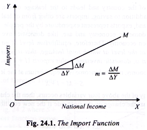
We have shown the import function in Fig. 24.1 where on the X-axis the level of national income and on the Y-axis imports of a country are measured. It will be seen that even at zero national income some imports are undertaken by exporting some capital accumulated in the past or by borrowing from abroad.

There are two concepts of propensity to import which should be understood. First, average propensity to import is defined as the proportion or percentage of national income spent on imports, that is, it is rupee value of imports divided by national income or M/Y.

Large countries such as the U.S.A., Russia and India have low average propensity to import and small countries such as Great Britain and Holland have high average propensity to import. The average propensity to import in India is between 0.02 and 0.03.

More important concept is the marginal propensity to import. The marginal propensity to import measures the change in import as a result of increase in national incomes and is algebraically expressed as ΔM/ΔY where ΔM is the change in value of imports and ΔY is the increase in national income. If imports increase by Rs. 3 when national income rises by Rs. 100, the marginal propensity to import (ΔM/ΔI) will be equal to 3/100 = 0.03 or 3 per cent. If increase in income by Rs. 100 leads to the increase in imports by Rs. 10, the marginal propensity to imports is 10/100 = 0.1 or 10 per cent.

The Foreign Trade Multiplier in an Open Economy:

In a closed economy equilibrium level of national income is determined at the level where intended saving equals intended investment (S = I). Saving represents leakage or withdrawal of some money from the income flow, while investment is the injection of some money into the income stream.

The level of national income is in equilibrium (that is, circular flow of income is constant) when leakage from the income stream in the form of savings is equal to the injection of investment expenditure. In an open economy, the role of foreign trade, that is, exports and imports of a country are also to be considered. Imports by consumers of a country represent the expenditure on imported goods by the residents of the country and leads to the leakage of some income from domestic economy.

Therefore, in addition to saving, imports are other form of leakage that occur in an open economy. On the other hand, exports represent expenditure by the people of foreign countries on the goods produced in the domestic economy and are, like domestic investment, injection into the income stream of an open economy.

Therefore, equilibrium level of national income in an open economy is determined at the level at which total leakage, that is, savings plus imports (S + M) equal total injection, that is, domestic investment plus exports (I + X) into the income stream.

Thus, in an open economy, national income is in equilibrium at the level at which

S + M = I + X

When a change in any of the above four variables occurs, then the change on the left side of the above equation must equal the change on the right side if the new equilibrium is to be achieved.

Hence

ΔS + ΔM = ΔI + ΔX …(1)

Now, change in saving, ΔS = s. ΔY

Where s = marginal propensity to save and

ΔY= change in national income.

Likewise, change in imports, ΔM = m. ΔY

where m = marginal propensity to import.

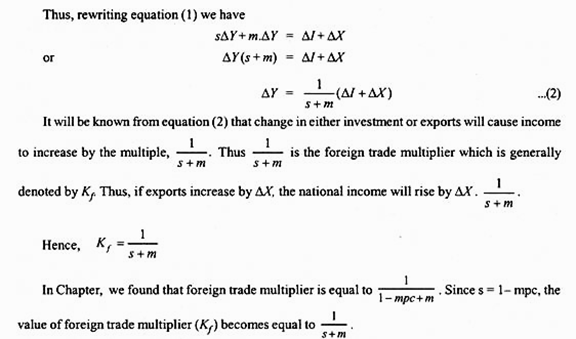
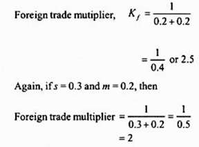
Thus, foreign trade multiplier is equal to the reciprocal of marginal propensity to save (s) plus marginal propensity to import (m). It is evident that smaller the leaks, that is, smaller the values of marginal propensity to save (s) and marginal propensity to import (m) the greater the value of foreign trade multiplier. Let us given an example. If s = 0.2 and m = 0.2, then

Graphic Representation of Foreign Trade Multiplier:

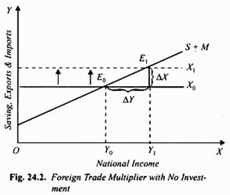
The foreign trade multiplier has been graphically illustrated in Fig. 24.2 where S + M is the saving plus import function curve and X₀ is the export curve which is constant as it has been assumed to be an autonomous variable, that is, independent of the level of income. To simplify our analysis we assume that there is no investment, equilibrium level of national income will therefore be deter­mined by consumption (saving) and exports.

Initially, the economy is in equilibrium at level of income Y₀ where S + M=X₀, investment being zero. Suppose there is autonomous increase in exports so that export curve shifts upward from X₀ to X₁. It will be seen from Fig. 24.2 that equilibrium income increases to Y₁.

Thus, increase in exports (ΔX) has led to the increase in income (ΔY) equal to Y₁ – Y₀ which is much greater than change in exports (ΔX). The expression ΔY/ΔX represents the foreign trade multiplier whose value depends on the slope of saving-import function curve S+ M which is equal to the reciprocal of the sum of marginal propensity to save and marginal propensity to import (1/s + m).

How the Foreign Trade Multiplier Works?

The foreign trade multiplier works in the same way as Keynes’ investment multiplier. When there is increase in exports, it will cause the increase in income of the exporters and those employed in the export industries. They will save some of the increase in their incomes and will spend a good part of the increases in their incomes on consumer goods, both domestic and imported ones.

While savings do not generate further income and represent leakage from the income stream, expenditure on im­ports leads to the increase in the incomes of the foreign countries from which goods are imported. Thus expenditure on imports also represents a leakage from the income stream as far as domestic economy is concerned.

But the increased expenditure on domestic goods as a result of increase in exports will go on increasing incomes in various successive rounds of spending till the multiplier fully works itself out.

It may be noted that increase in exports of a country can occur due to several reasons. There may be change in tastes or demand of the people of foreign countries for goods of a country. To begin with, the exporters may meet the demand for exported goods by selling their inventories and enjoy higher incomes.

But in the next periods, they will make efforts to increase the production of exported goods and employ more workers. This will generate new income and employment in the export industries. But the working of multiplier does not stop here.

Those employed in export industries will spend a good part of their increased incomes on goods produced by other industries and in this way increases in income, production and employment will spread in the whole of the domestic economy.

The Foreign Trade Multiplier: With both Exports and Domestic Investment:

In our foregoing analysis we have explained the multiplier effect of autonomous increase in exports assuming that there is no domestic investment. We will now further elaborate the foreign trade multiplier by considering both exports and domestic investment.

In an open economy when there is positive investment the level of equilibrium in national income is reached when sum of domestic investment and net exports equals saving.

Thus, in an open economy the condition for the equilibrium level of national income is:

I_d + X_n = S …(1)

where I_d is domestic investment, X_n is net exports and S is the saving

Net exports (X_n) is the net of exports over imports, that is, X_n = X – M

Substituting X – M for X_n in equation (1) we get

I_d + (X – M) = S

or I_d + X = S + M

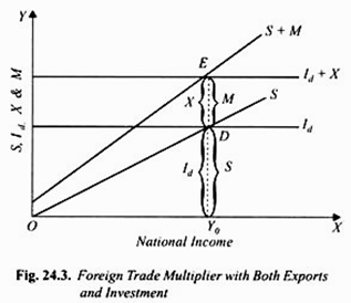
In the case when there is positive domestic investment the determination of the equilibrium level of national income is graphically shown in Fig. 24.3. The curve I_d represents autonomous domestic investment which remains constant. S is the saving function curve showing that saving is the increasing function of income.

Over the domestic investment curve (I_d) we have added the exports (X) of the economy to get I_d + X curve. To the saving function curve we have added the import function curve to obtain the aggregate of saving and import functions curve (S + M).

It will be observed from Fig. 24.3. That I_d + X equals S+M at point E and thus the equilibrium level of national income Y₀ is determined. Note that at Y₀ level of income saving (S) and domes­tic investment (I_d) are also equal. Thus, at equilibrium income Y₀:

I_d + X = S + M

and I_d = S

Therefore, at Y₀ equilibrium income:

X = M

The equality of exports (X) with imports (M) implies that there is equilibrium in the balance on the current account. However, it is important to note that it is not necessary that at equilibrium level of national income exports (X) equal imports (M).

This equilibrium in the current account balance along with equilibrium of saving and domestic investment occurs only when exports are equal to imports at the equilibrium level of income determined by the equality of saving and domestic investment.

In Fig. 24.3. at equilibrium income Y₀ at which saving equals domestic investment, imports are equal to DE. If exports happen to be equal to DE, the equilibrium in the current account balance will also occur. However, this is not necessary because exports may be greater or less than the imports DE.

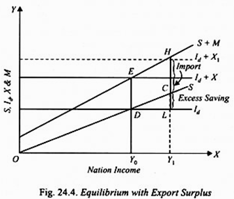
Suppose autonomous exports increase so that the investment – exports curve shifts above to I_d + X₁ as shown in Figure 24.4. This new I_d + X₁ curve intersects S + M curve at point H and as a result equilibrium national income Y₁ is determined. It will be seen from Fig. 24.4 that at national income Y₁ the volume of exports is LH which exceeds the imports CH by LC amount.

Note that LC is the amount by which saving exceeds domestic investment. It is this excess of saving over domestic investment that maintain the equation l_d + X = S + M despite exports (X) being not equal to imports (M). Thus, in this case there is surplus in the balance of payments on current account.

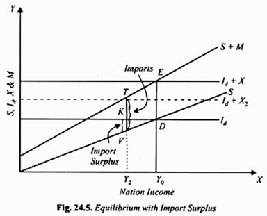
The opposite case can also occur when exports fall below ED. If the exports fall and the in­vestment-export curve shifts to l_d + X₂ (Fig. 24.5), the new equi­librium is reached at income level Y₂ at which I_d+X₂ = S + M. In this equilibrium situation imports are equal to VT which exceeds ex­ports (X₂) which are equal to KT.

Thus, though the open economy is in equilibrium as l_d + X₂ = S + M at income level Y₂, there exists import surplus or deficit in current account balance which again implies that there is disequilibrium in the balance of payment on the current count.

However, in this case of import surplus (i.e. deficit in current account balance), domestic investment must exceed domestic saving by an equal amount so as to maintain the equality of I_d + X with S + M. This is possible only if a country borrows from abroad to keep investment greater than domestic savings.

The above analysis shows that while the open economy as a whole may be in equilibrium, it is not necessary that balance of payment (on current account) will also be in equilibrium.

Increase in Imports: The Reverse Working of Foreign Trade Multiplier:

Whereas increase in exports has an expansionary effect on national income, the increase in imports will have opposite effect on national income. Imports will bring about contraction in national income. Further, the effect of increase in imports on national income will not be equal to the increase in imports but will have a multiplier effect in reducing national income.

There can be several reasons for the increase in imports of a country. An important reason for the increase in imports is the change in tastes or preferences of the people. The people of a country may have started preferring the imported goods as compared to Swadeshi (home produced) goods.

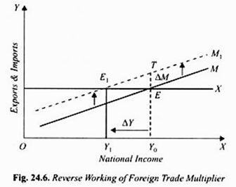
The reduction in import duties on the imports and thus making them cheaper may be another reason for the increase in imports a country. The contractionary effect of increase in imports on the income and employment in a country is illustrated in Fig. 24.6. To simplify our analysis we have assumed that there are no net savings and investment.

In this Fig. 24.6 the export curve is a horizontal straight line since exports are assumed to be autonomous of changes in national income. The curve M represents the import function curve which slopes upward showing that it changes with national income.

The two curves X and M inter­sect at point E and determine Y₀ equilibrium level of national income. Now suppose that there is increase in imports (ΔM = ET), say due to the change in preferences for foreign goods, and as a result import function curve shifts above to the position M₁, the export curve X remaining un­changed.

It will seen from Fig. 24.6 that new import function curve M₁ and export curve X intersect at point E₁ and as result the equilibrium level of income falls to Y₁. Note that reduction in income is greater than the increase in imports; ΔY is much greater than ΔM. This is due to the working of foreign trade mul­tiplier which in the present case works to reduce income.

When the consumers buy more foreign goods and less domestically produced goods, the demand for domesti­cally produced goods decreases which result in fall in incomes and employment of those engaged in the domestic indus­tries. These reduced incomes further re­duce the expenditure on the purchase of other home-produced goods and so on. The reverse process of contraction of in­come, production and employment goes on till the multiplier fully works itself out.

It is important to note that initial attempt to increase imports has not finally resulted in any increase in imports. Imports Y₀E at the initial equilibrium income Y₀ are equal to imports Y₁E₁ in the new equilibrium at the much lower level of income. This is another paradox which is described as import paradox.

What has actually happened is that the increase in imports and consequent upward shift in the import function leads to a large contraction in income through the reverse working of foreign trade multiplier so that in the new equilibrium at a much lower income, less is imported. This is generally referred to as income effect.