R.M. Solow’s Model (With Diagram)

Read this article to learn about the R.M. Solow’s model in neo-classical theory of economic growth.

Robert M. Solow to Massachusetts Institute of Technology (MIT) in his paper “A contribution of the Theory of Economic Growth”—in the Quarterly Journal of Economies, LXX (February, 1956) developed a model of economic growth called a neo-classical model of economic growth.

Dr. Solow shows that H-D model about steady growth has limited value even for developed economies. He finds fault in H-D models in as much as they are based on constant capital-output ratio.

The assumption of fixed proportions and constant capital output ratio are given up by Solow as indeed by other neo-classical economists also. Since the technical coefficients change both in the capital intensive as well as labour- intensive sectors, his model can be used for underdeveloped countries also. Substitutability between capital and labour plays a central role in Solow’s model.

Solow retains Harrod’s assumptions of a constant saving ratio and shows that on account of the substitutability of factors for each other in production, by increasing the labour capital ratio—the output-capital ratio can be increased and hence the warranted rate of growth (G_w) can be made equal to the natural rate of growth (G_n) and the equilibrium path is or becomes stable. Besides, the attempts of Mrs. Robinson, Meade, Kaldor— Solow’s model is another attempt to extend and modify the H-D models.

There are a number of growth models where C/O ratio is taken as a variable and not a constant as in H-D models—these models have been built by Samuelson, Solow and Swan. These are known as neo-classical growth models because they postulate a continuous production function with increasing (and not fixed) C/O ratio.

It is based on certain assumptions which are as follows:

(a) Production of one commodity.

(b) Constant returns to scale. In other words, production function is homogeneous of the first degree.

(c) There are mainly two factors, L and K which act as inputs and they are paid according to their Marginal Physical Productivities (MPP).

(d) Prices and wages are flexible.

(e) Output is net output after making allowance for depreciation of capital, that is, it is net of depreciation.

(f) Labour and capital can be substituted for each other.

(g) There is full employment of labour and available stock of capital.

Given these assumptions, Solow tries to show that with variable technical coefficient there will be a tendency for capital labour ratio to adjust itself through time in the direction of equilibrium ratio. If the initial ratio of capital to labour is more, capital and output would grow more slowly than labour force and vice versa. Solow’s analysis converges towards equilibrium path (steady state) to start with any capital labour ratio.

The essence of Solow, Swan models is that these models avoid the problem which arises in H- D models—if the natural and warranted rates of growth diverge. Solow’s model does this through the variation in C/O ratio, it allows the warranted rate of growth to vary through changes in C/O ratio. It also means changes in S (saving) are not so relevant.

Changes in warranted rate of growth result from changes in (C/O) and not in S. What this model does is to lay down the mechanism that if capital growing faster than population, then the two can be brought back into equilibrium by increasing capital intensity of production. Similarly, if capital is increasing less rapidly than population, full employment equilibrium can be brought about by reducing the capital intensity of production. Thus, it is through the variations of (C/O) ratio that balanced growth full employment equilibrium is achieved. In developing his analysis, Solow uses Harrod’s methodology.

Harrod’s model had a knife-edge balance in the long run economic system, where saving ratio (S), the capital output ratio (C/O), the rate of increase of the labour force are the key parameters. If the magnitudes of these parameters were to slip even slightly from the dead centre, the consequences will be either growing unemployment or inflation. In his system G_n depends on the increase of the labour force and G_w depends on the savings and investment habits of households and firms. Solow and Swan models provided the basic outlines of the neo-classical solution of Harrod’s twin problems of the discrepancy between the warranted and the natural rates of growth and the instability of the capitalist system.

It was because of the weakness of the H-D model of growth that led economists to explore more complex theories which allowed for variations in labour as well as capital and substitution of labour and capital for each other. Solow was one of the first to work along these lines. With variable factor proportions and flexible factor prices, he showed that the growth path was not inherently unstable. If labour force was more than the supply of capital, the price of labour will fall relative to the rate of interest or if capital is more than labour, the price of labour would rise.

Variations in factor prices and factor substitution will mitigate the hardships of the likely departure from the H-D growth path. One production function explored by Solow which permitted capital and labour to grow at different rates was the Cobb-Douglas production function.

In equation form this is:

Y = yK ^αL ^β

where Y, K and L are output (income), capital and labour ; y is a constant, different for different economies ; and a and P are exponents which indicate the marginal efficiency of capital and labour. In the Cobb-Douglas function α and β add¹ to 1 which means that increases in income are exactly equal to the marginal physical productivity (MPP) of the factors times their respective increases.

This implies constant returns to scale—a departure from the classical diminishing returns. Thus, in Solow’s model, once we know the time path of capital stock and that of labour force, we can compute from the production function the corresponding time path of real income or output. The marginal productivity equation determined the time path of the real wage rate.

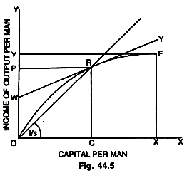
Let us look at the problem in more details. We are postulating a continuous production function linking output to the inputs of capital and labour, while there are constant returns to scale and no technological progress, so that G_y = G_n. All that we have to see is, how an alteration in the C/O ratio allows the rate of growth (G_v) to rise to the required level of population growth (G_n). If the economy has to be in equilibrium at full employment, we must have G_n= s/v, because we are assuming absence of technical progress, therefore, the rate of increase in the labour force equals the natural rate of growth, so that I = s/v or v = (where v is the C/O ratio and s is the saving income ratio). Since s and I are given and constant, we have to know, that level of which v is consistent with this level of s/l. It is done with the help of the given Fig. 44.5.

On the X-axis in the Fig. 44.5, capital per man and on the Y-axis, output (income) per man is shown. The production function is shown by OF. It shows what income per head will be at all levels of capital per head. With no capital, income is zero. As capital per head increases, increase in income per head declines and finally, with a capital per head of OX, income or output per head is OY.

Beyond F, the production function is horizontal. The line OR cuts OF at R and the line WT is tangent to OF at R. The slope of the line OR shows income per head divided by capital per head. It shows the C/O ratio required for G_w to equal G_n (given the saving ratio of the community). Symbolically, it shows Y/L K/L= Y/L.L/K=Y/K. Now Y/K is the inverse of the C/O ratio. Since, v = s/l, therefore, 1/v= s/I

The slope of OR is, therefore, I/s = l/v. Since, I is the natural rate of growth (because there is no technical progress) and s/v is the warranted rate of growth, we can see that G_n = G_w at point R (if s/l = l/v, then v = s/l). This means, in other words, that the slope of OR is determined (or depends upon) by the proportion of income saved and the growth of the labour force (as indicated by the angle l/s in the Fig. 44.5).

Whereas the slope of WT, the tangent at R to the production function OF, shows the marginal product of capital at R. In other words, it shows the rate of profit at R, which is required by the levels of s and I. It shows the additional income derived from a small increase in capital. If we extend the tangent at R back to touch the Y-axis at W, then WP shows the share of profit in income OP. It shows capital per head (OC) multiplied by the rate of profit (r). The remainder of income OW goes to wages, wage per man is OW. Thus, R is a point where all the elements in the model are G_n= s/v= G_v this is the essence of Solow’s Model.

Possible Growth Paths:

Prof. Solow has introduced a basic equation to show whether there is always capital accumulation consistent with any rate of growth of the labour force towards a steady state.

Prof. Solow’s fundamental equation is as follow:

r = sF(r, I) – nr

In this equation r is the ratio of capital to labour (K/L), n is the relative rate of change of the labour force (L/L). The function F(r, I) shows output per worker as a function of capital per worker. In other words, it is the total product curve as different amounts of r of capital are employed with one unit of labour.

The equation itself states or implies that the rate of change of capital-labour ratio (r) is the difference of two terms, one showing the increment of capital [sF (r, I)] and the other increment of labour (nr). Solow has made study of growth patterns of population and uses various diagrams to illustrate possible growth patterns based on his above fundamental equation. It is illustrated with the help of the diagram.

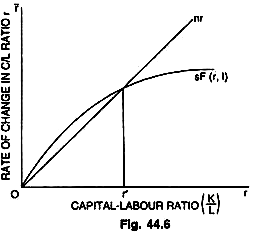
Solow treats the population growth as a function of per capita income (and so of the capital labour ratio) instead of treating it as an autonomous variable. On the horizontal axis in the Fig. 44.6 given here is measured r, the ratio of capital to labour (K/L). On the vertical axis is measured r, the rate of change in the capital-labour ratio through time. Population growth is shown by n and it is shown as a function of capital per head r.

The pattern of population growth implied in this diagram is that “for very low levels of income per head or real wage, population tends to decrease, for higher levels of income it begins to increase and that for still higher levels of income, the rate of population growth levels off and starts to decline.” The other curve in this figure is sF (r, I).

It is a capital accumulation function, it makes the rate of increase in capital per head depend on the relation of output per worker to capital per worker. It is so drawn as to show the diminishing marginal productivity of capital. At the point of intersection of the two curves nr = sF (r, I) and r = 0. By drawing a perpendicular from the point of intersection of the two curves on horizontal base, we get r ‘determining the capital-labour ratio at r’, which is bound to be constant because r = 0.

Now, should the capital labour ratio at r’ be ever established, it will be maintained and the capital stock must expand at the same rate as the labour force and capital and labour will grow in proportion. Assuming, constant returns to scale, the real output will also grow at the same relative rate n, and output per head of labour force will be constant.

What will happen if r and r’ are not equal? What will be the behaviour of the capital-labour ratio if there is a divergence between r’ and r? In case r > r ‘then nr > sF (r, I) and this will make r to decrease back to r’. In the opposite case, if r < r’ then nr < sF (r, I), and r will increase towards r’. Thus, the equilibrium value r’ is stable. Whatever the initial value of the capital labour ratio, the system will develop towards a state of balanced growth at the natural rate.

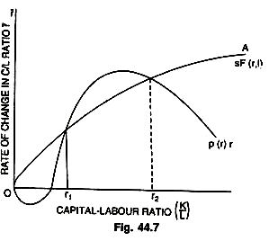
If the initial capital stock is below the equilibrium ratio, capital and output will grow at a faster rate than the labour force until the equilibrium ratio is established. If the initial ratio is above the equilibrium value, capital and output will grow more slowly than the labour force. The growth of output is always intermediate between those of labour and capital. However, the strong stability as shown in Fig. 44.7 is not inevitable. It all depends upon the shape of the productivity curve sF (r, I). The Fig. 44,7 gives a more realistic path.

In the Figure, horizontal axis measures ratio of capital to labour (K/L) and vertical axis measures the rate of change in the rate of capital to labour ratio (r), n represents population growth as a function of capital per head (r). The curve, 4 is capital accumulation function, i.e., sF(r, I). At any initial ratio of capita to labour below r₂, the system will revert back to equilibrium at the low ratio of capital to labour, r₁—-with the correspondingly low rate of increase of output.

If we start with a capital labour ratio anywhere below r₂ the only way to assure cumulative growth is to make a sudden jump to a ratio of capital to labour above r₂. This clearly shows that a gradual approach to r₂ is unlikely to be effective. Prof. Solow concludes “that when production takes place under the usual neo-classical conditions of variable proportions and constant returns to scale, no simple opposition between natural and warranted rates of growth is possible. There may not be any knife-edge. The system can adjust to any given rate of growth of the labour force, and eventually approach a state of steady proportional expansion”, that is:

Critical Evaluation:

Solow says that it is very difficult to contemplate systematic conclusions from changes over time in the production function. However, Solow’s model demonstrates that as long as real income is positive, positive net capital formation must result. This rules out the possibility of a Ricardo-Mill type classical stationary state and suggests the experiment of letting the rate of saving depend on the yield of capital, for the saving ratio need not go to zero.

In Solow’s own words, “My purpose was to examine what might be called the tight rope view of economic growth and to see where more flexible assumptions about production would lead to a rather simple model”. The policy implication of Solow’s model is that if there is a rise in the real wage rate corresponding to a capital-labour ratio without arise in productivity and rise in capital, it will bring unemployment and vice-versa.

Solow is one of the pioneers in developing a neo-classical model with the help of a neo-classical production function. The assumption of substitutability between labour and capital in the process of growth provides a touch of realism. The reason that the Solow’s model is stable and the Harrod’s model is unstable is not because Solow allows for the substitution of capital for labour, but because of different assumptions about dynamic adjustments and the determination of aggregate output. While Solow assumes that output is determined by the factor supplies, Harrod assumes that entrepreneurs themselves determine the level of aggregate output (constrained, of course, by the factor supplies).

Thus, while the changes in output in the Solow’s model depend simply on changes in factor supplies (in the absence of technological changes), changes in output in the Harrod’s model depend on particular assumptions about entrepreneurial behaviour and expectations.

Despite the merits of Solow’s model, it has been found weak in many respects. Solow’s model does consider the problem of the balance between G_w and G_n but does not consider the problem of the balance between G and G_w. Again, in Solow’s model we note the absence of investment function and once it is brought into the picture the Harrodian type of instability also reappears.

Domar has rightly observed, “The use of growth model as a practical guide to economic development is enticing but the pitfalls are deep indeed. The rate of growth of output is expressed in our models essentially as a function of the propensity to save and the capital coefficient (in one form or another). Given only slightly optimistic, but plausible magnitudes of these two parameters, economic development seems assured—on paper of course ! Both are most heroic abstractions implying a long list of assumptions about the actual working of the economy which these parameters, in their simple innocence conceal.”